How to Use Formula in Excel Table (4 Suitable Examples)

Excel Table allows you to create formulas that apply to the entire table, copy easily, and are more options than traditional formulas which are called structured references. This article will help you understand all the amazing features of Excel Tables and will convince you to use formula in Excel Table.

Download Practice Book

You can download the free Excel template from here and practice on your own.

What is an Excel Table?

We can say that Excel Tables are containers for our data. Imagine you have a storeroom, so there you will arrange your books to a shelf, electric tools to a different shelf. Excel Tables are like those shelves. It helps to contain and organize data in your worksheets like that. Tables manage excel that all the data is related.

Create a Formula and Apply to an Excel Table

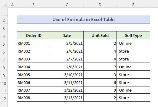
The way we use an Excel formula in a typical Excel sheet and in an Excel Table is a bit different but not so difficult. I’ll show some easy examples which will be well enough to learn that. Let’s start with the SUM function. Before that, I’ll introduce you to my dataset first. It represents selling information- Order ID, Date, Unit Sold, and Sell Type of a company.

At first, we’ll convert our dataset to a table.

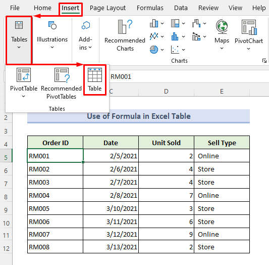
Step 1:

⏩ Select any cell from the dataset.

⏩ Then click as follows: Insert > Tables > Table

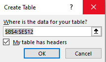
Step 2:

⏩ Now just press OK here.

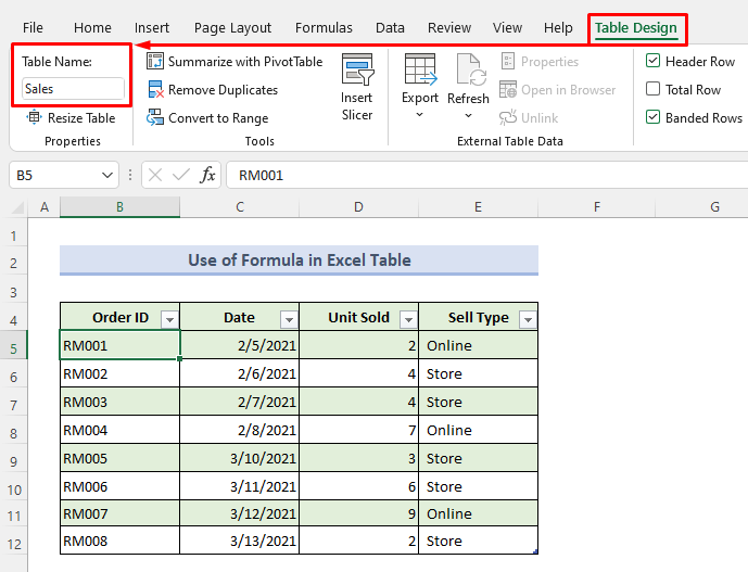
Look that our table is ready. I have changed the name of the table to ‘Sales’. To do that-

Step 3:

⏩ Press any data in the table and click- Table Design > Table Name

Now let’s count the total sold unit with the SUM function.

Step 4:

⏩ Activate Cell D14.

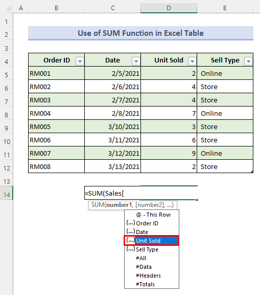
⏩ Type =SUM(Sales[

Then you will see that it is showing the header names of our table like the image below.

⏩ Select Unit Sold.

It’s called the Structured Reference. No need to use the cell references here.

Step 5:

⏩ Finally, close the brackets and hit the Enter button.

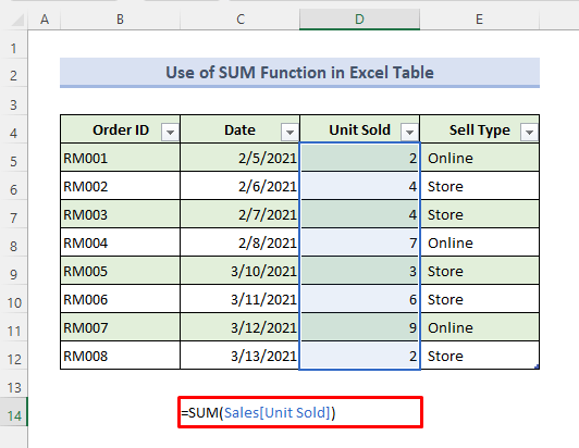
And now we have got our total sold unit.

Calculate Total Cost:

Next, I’ll show how to use the total column in a formula. For that, I have modified the table. I have added products’ prices and their delivery costs. Then to calculate the total I have added a new column.

Steps:

⏩ Type the name of the column adjacent to the last header and hit the Enter button, Excel Table will automatically convert it to a part of the table.

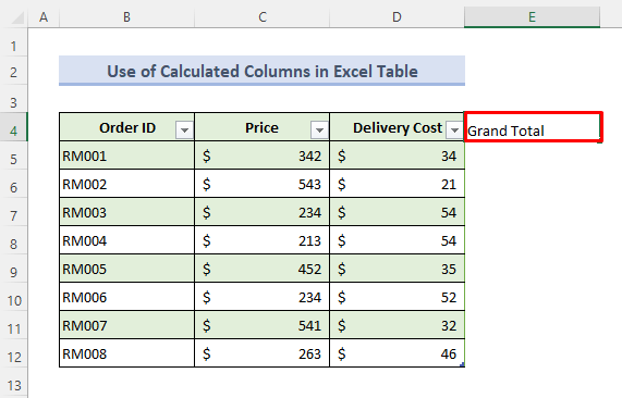
Here’s our new column.

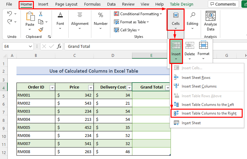
Also, you can click- Home > Cells > Insert > Insert Table Columns to the Right to add a column.

Now we’ll find the total cost for each order using Structured Reference.

Steps:

⏩ In Cell E5 type the formula given below-

⏩ Press the Enter button on your keyboard.

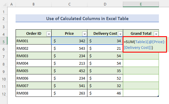
Now take a look that we have found the total values for all rows. No need to use the Fill Handle tool here. It’s the advantage of Excel Table.

Read More: Create Table in Excel Using Shortcut (8 Methods)

3 More Examples with Formula in an Excel Table

Let’s see three more examples of how to use formulas in an Excel Table.

1. SUMIF Formula with Single Criteria

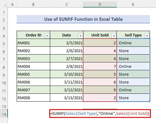
Let, we’ll count the sold units which have been sold in online with the SUMIF function. The SUMIF function returns the sum of cells that meet a single condition.

Steps:

⏩ Type the given formula in Cell D14–

⏩ Click the Enter button then.

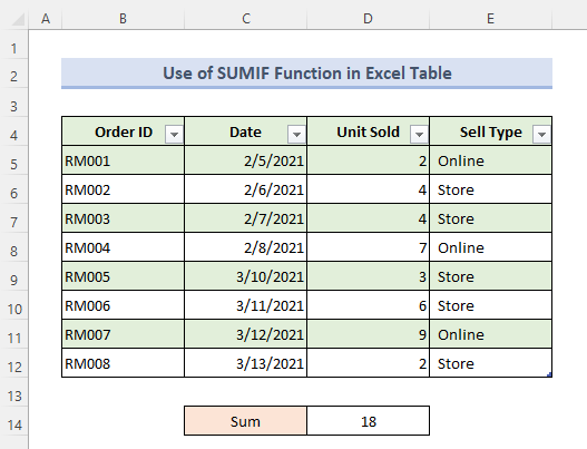
Here’s our output-

Read More: How to Use an Excel Table with VBA (9 Possible Ways)

Similar Readings

• How to Make a Table in Excel (With Customization)
• Use Calculated Field in Excel Pivot Table (8 Ways)
• Calculated Field Sum Divided by Count in Pivot Table
• How to Use Excel Table Reference (10 Examples)
• Excel VBA Code for Each Row in a Table (Add, Overwrite, Delete, etc.)

2. SUMIFS Formula with Multiple Criteria

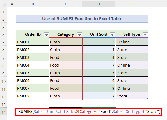
Here, we’ll count units with multiple criteria. We’ll count only those units which are Food items and sold in-store by using the SUMIFS function. The SUMIFS function returns the sum of cells that meet multiple conditions.

Steps:

⏩ By activating Cell D14 write the given formula-

⏩ Later, just hit the Enter button.

We are done with the operation now.

Read More: Does TABLE Function Exist in Excel?

3. COUNTIF Formula to Count Based on Criteria

In our very last example, we’ll count the online orders with the COUNTIF function. The COUNTIF function counts the number of cells in a range, that meets the given criteria.

Steps:

⏩ Write the given formula in Cell D14–

⏩ Hit the Enter button to get the result.

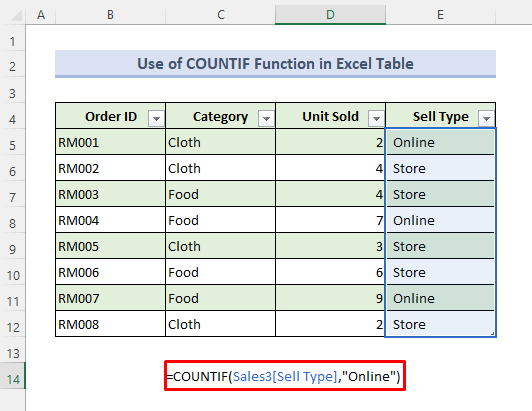
Then we’ll get the output like the image below.

Read More: [Fix]: Formulas Not Copying Down in Excel Table (3 Solutions)

Conclusion

I hope all of the methods described above will be good enough to use a formula in an Excel table. Feel free to ask any question in the comment section and please give me feedback.

Related Articles

• How to Edit a Pivot Table in Excel (5 Methods)
• Refresh All Pivot Tables in Excel (3 Ways)
• Types of Tables in Excel: A Complete Overview
• Convert Range to Table in Excel (5 Easy Methods)
• Reference Table Column by Name with VBA in Excel (6 Criteria)
• How to Provide Table Reference in Another Sheet in Excel