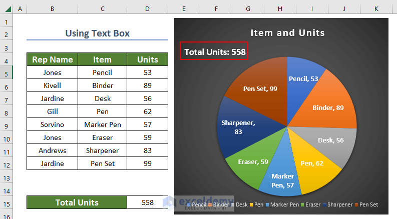
How to Show Total in Excel Pie Chart: 2 Effective Ways

Method 1 – Using Text Box in Pie Chart to Show Total

Step 1: Inserting Pie Chart

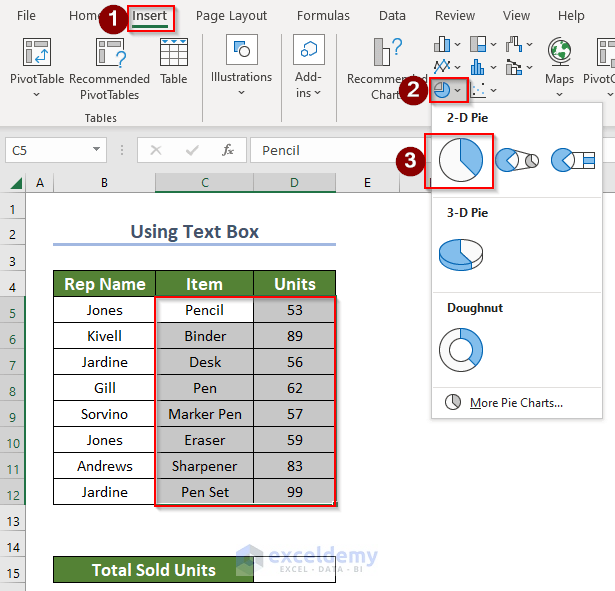
Select the preferred range for which you want to create the Pie Chart. In this dataset, C5:D12 is the preferred range that we are creating the Pie Chart.
Go to the Insert tab and click on Pie Chart drop-down. The drop-down list has 3 sections which are 2-D pie, 3-D pie, and Doughnut.
Click on 2-D Pie.

A Pie Chart will be generated in your worksheet.
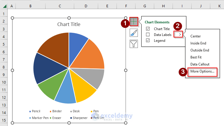
Click on the chart and then click the plus symbol, which is Chart Elements.
Click the arrow sign (>) beside Data Labels.
Click on More Options.

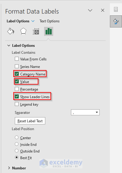
After clicking More Options, you will get the Format Data Labels dialog box.
Select Category Name, Value, and Show Leader Lines from Label Options.
Close the Format Data Labels dialog box.

You can edit the Chart Title and give your preferred Chart Title. It is the Item and Units.

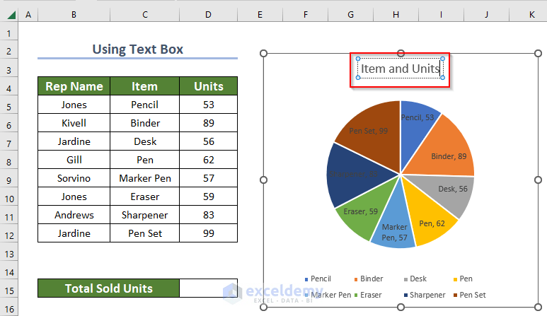
Format the font size, and color.

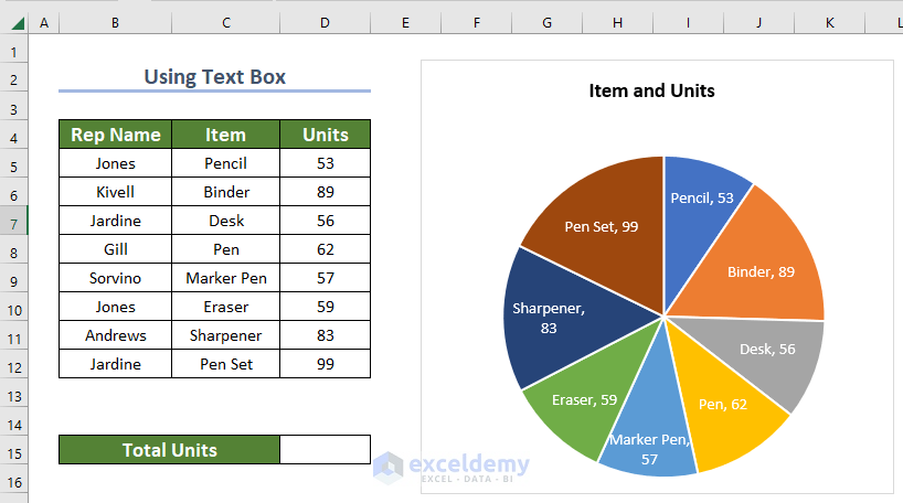
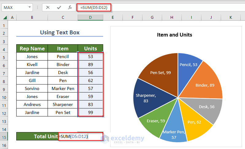
Step 2 – Calculating Total Units

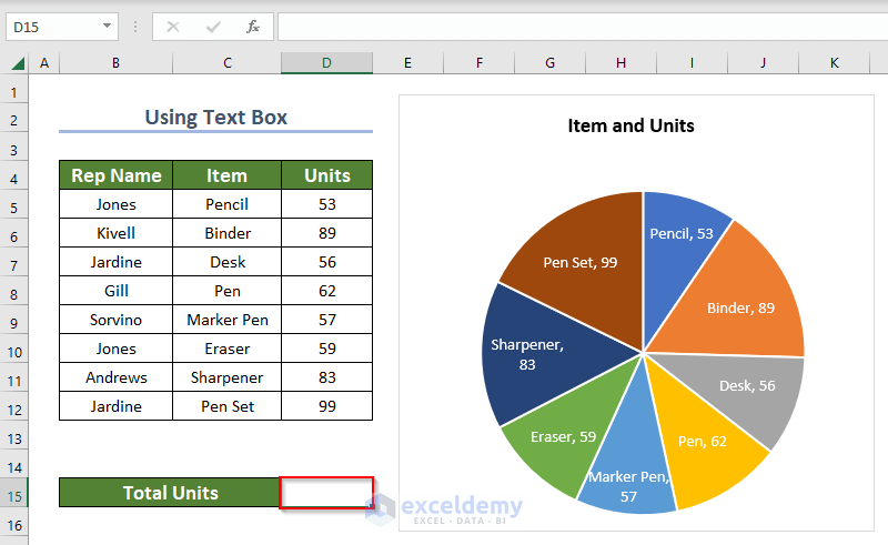
Select your preferred cell to get the output. We selected cell D15 in this case.

Select cell D15 and then type the following formula:

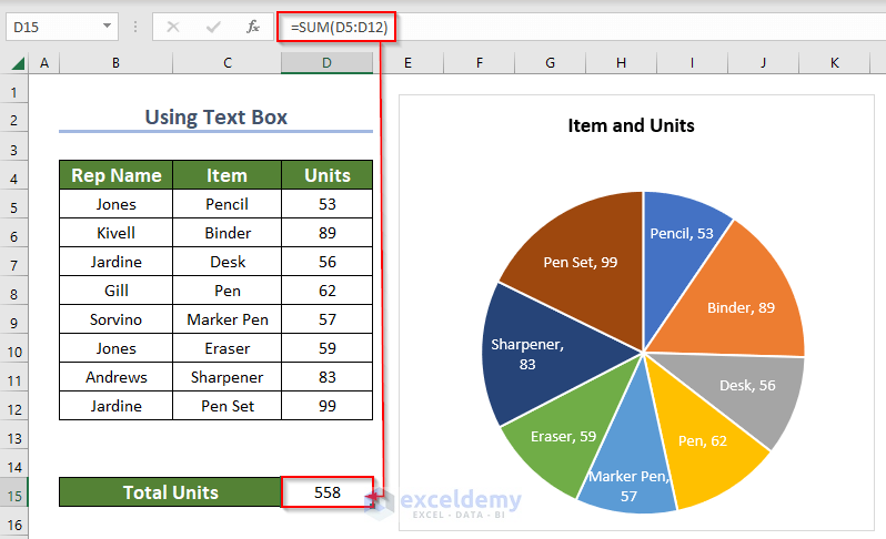
=SUM(D5:D12)

The SUM function will return the sum of the cell values in the defined range. It performs the mathematical operation of addition. In this case, D5:D12 is the range of values.

Press ENTER key and the result will be shown in cell D15.

Step 3 – Employing Text Box to Show Total Units

Insert a text box where you want to display the total. Click on your pie chart and go to the Insert menu.
Select the Text Box.

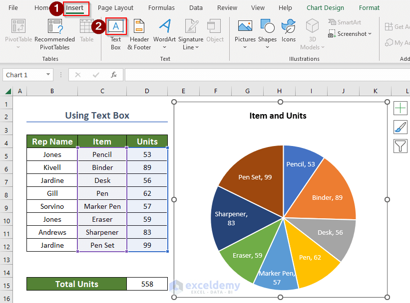
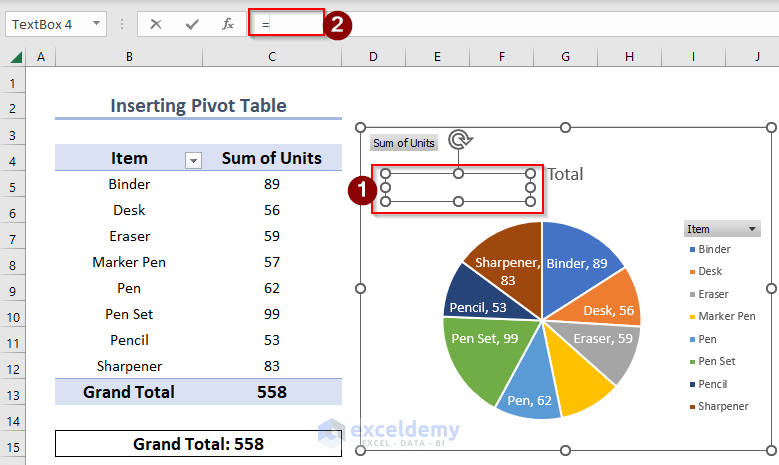
Draw a Text Box on the chart at the point where you want the total to be displayed.

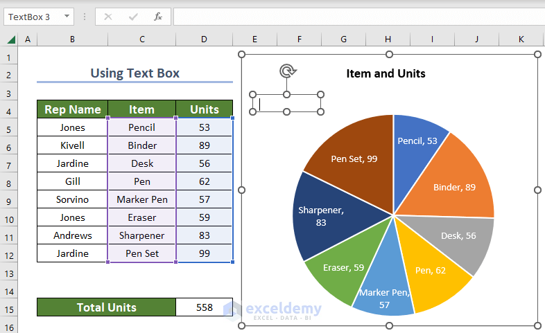
The Text Box still open/active, type an Equal sign (=) in the Formula Bar.

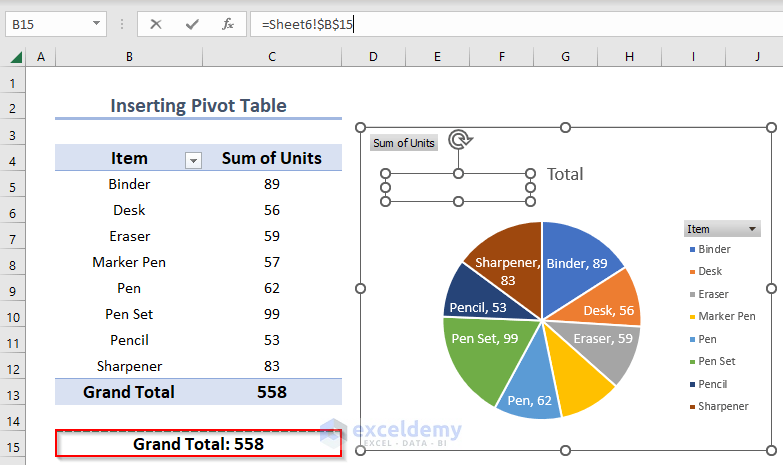
Select the cell that contains the data that you want to display in the Text Box on the chart. It is cell D15.

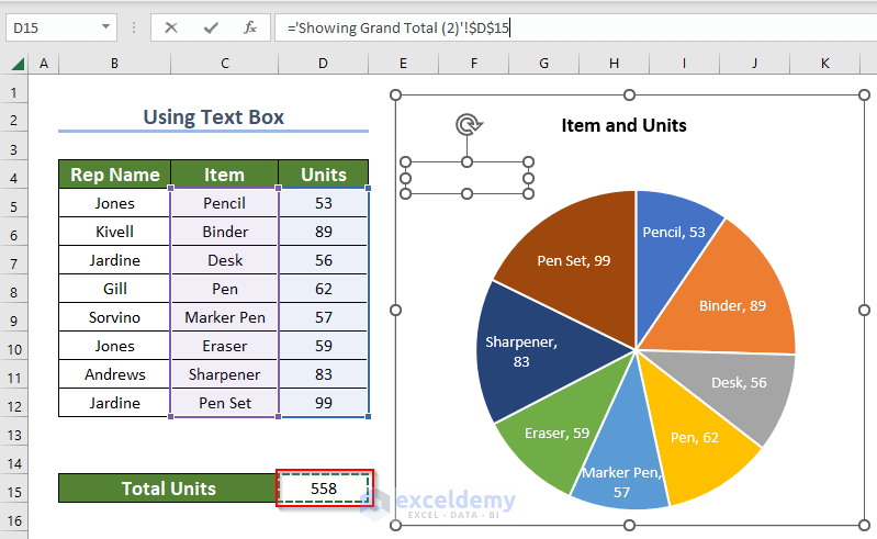
Press ENTER.

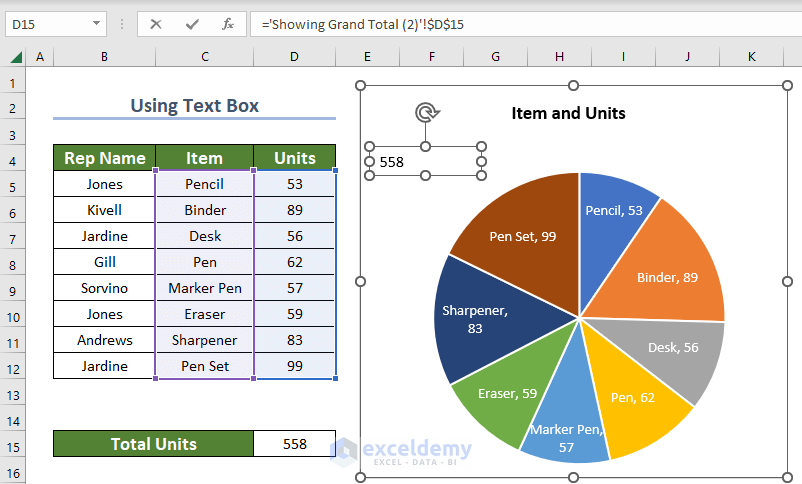
Format the font size, color, and theme color.

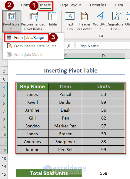
Method 2 – Showing Grand Total Using Pivot Table in Excel

Step 1: Inserting Pivot Table

Select the preferred range for which you want to create the PivotTable. In this dataset, B4:D12 is the preferred range that we are creating the PivotTable.
Go to the Insert tab.
Click on the PivotTable dropdown.
Select From Table/Range.

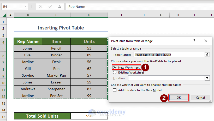
After selecting From Table/Range, a new window named PivotTable from table or range will pop up.
Select New Worksheet and click OK.

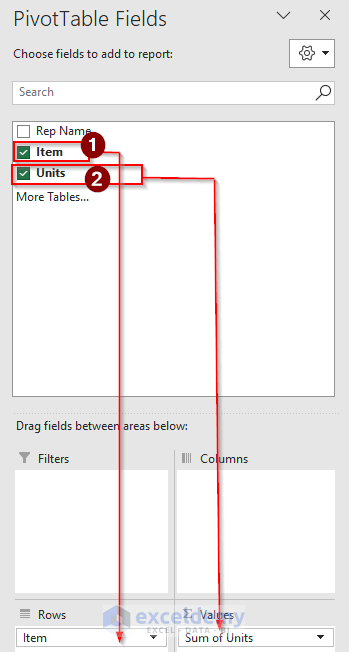
Excel will take you to a new worksheet and you will get the PivotTable Fields dialog box.

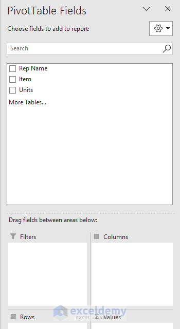
Select Item and Units and drag them to Rows and Values. We ignored Rep Name at this point to keep it short and simple for better understanding.

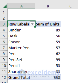
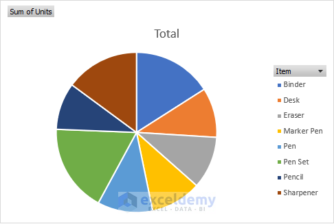
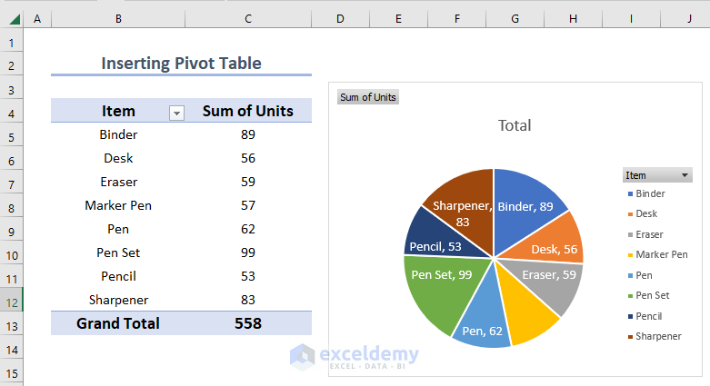
See a Pivot Table created in your worksheet with column names Row Labels, and Sum of Units.

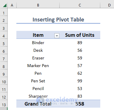
Adjust this PivotTable to your dataset’s column name. We named Row Labels to Item and adjusted font, heading, etc.

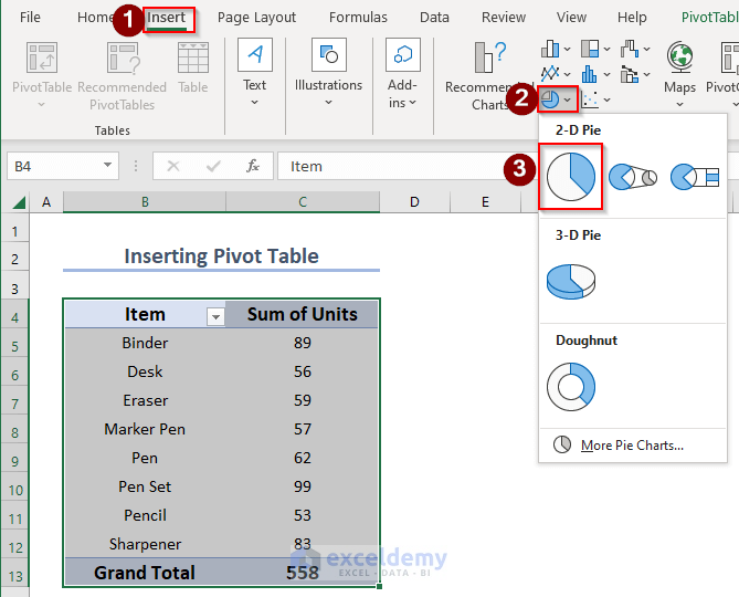
Step 2: Creating a Pie Chart

Select the range of the PivotTable and go to the Insert tab.
Click on the Pie Chart drop-down and select 2-D Pie.

A Pie Chart will be generated in your same worksheet.

Follow Step 1 of Method 1 to add Legend and Data Labels to the Pie chart.
See the Pie chart with Legend and Data Labels.

Step 3: Employing Total to Pie Chart

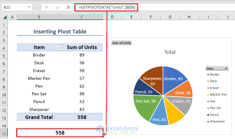
Select cell B15 and type an Equal sign (=) in cell B15.

In the worksheet, select the cell that contains the data and it will generate the following formula. It is cell C13.

=GETPIVOTDATA("Units",$B$4)

The GETPIVOTDATA function returns visible data from a PivotTable. GETPIVOTDATA(“Units”,$B$4) returns the total of Units. $B$4 is the reference to the starting cell of PivotTable.

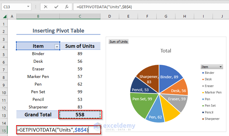
Press E.
NTER Key and the output will be shown in cell B15.

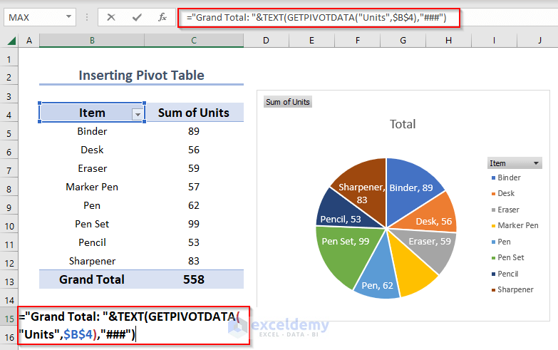
Adjust the formula like below

="Grand Total: "&TEXT(GETPIVOTDATA("Units",$B$4),"###")

The TEXT function enables you to modify the appearance of a number by applying formatting to it with format codes. It is useful when you want to combine a text or symbol with a number. To show “Grand Total:” in the PieChart we adjusted the formula with the Text Function.

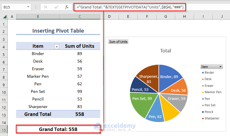
Press ENTER key and the output will be shown in cell B15.

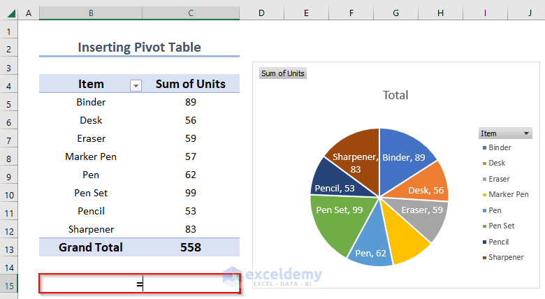
Insert a text box where you want to display the total. To do so, click on your pie chart and go to the Insert
Select the Text Box.

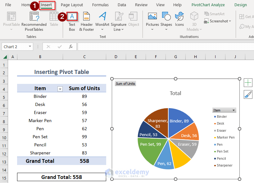
Draw a Text Box on the chart at the point where you want the total to be displayed.
With the Text Box still open/active, type an Equal sign (=) in the Formula Bar.

Then in the worksheet, select the cell that contains the data that you want to display in the Text Box on the chart. It is cell B15.

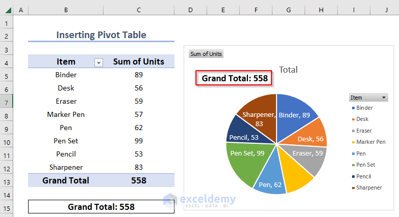
Press the ENTER key and you will see your Grand Total in your PieChart like below.

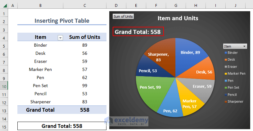
Adjust the font size, color, and theme color as you wish. You can also edit the Chart Title. We gave Item and Units as our Chart Title and changed the theme.

We have got our final Excel Pie Chart showing the total.

Download Practice Workbook

Showing Total in Pie Chart.xlsx

<< Go Back To Excel Pie Chart | Excel Charts | Learn Excel

Get FREE Advanced Excel Exercises with Solutions!