How to Show Percentage and Value in Excel Pie Chart

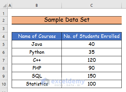
To demonstrate how to show Percentage and Value in an Excel Pie Chart, we’ll use the following sample dataset:

Step 1 – Selecting the Dataset

• Select all the columns in the given dataset.

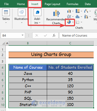
Step 2 – Using Charts Group

• Select the Insert tab.
• Select the Insert Pie Chart command from the Charts group.

Read More: [Solved]: Excel Pie Chart Not Grouping Data

Step 3 – Creating the Pie Chart

• Select the 2-D Pie Chart option.

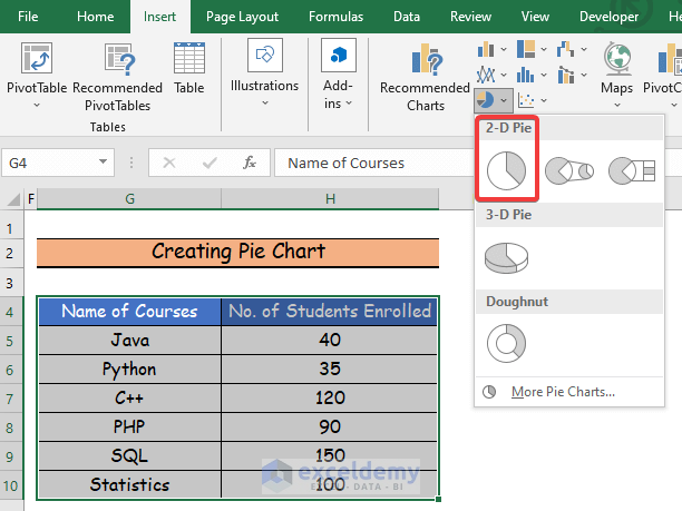
The pie chart below is generated.

Read More: How to Show Percentage in Legend in Excel Pie Chart

Step 4 – Applying Format Data Labels

• Click the Chart Element icon.
• Check the Data Labels option.

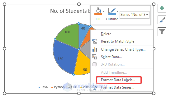
The data values for each segment now display in the pie chart.

• Right-click on the pie chart.
• Select the Format Data Labels command.

• Check the Value and Percentage options.
• Choose any of the Label Position options. Here, we select Best Fit.

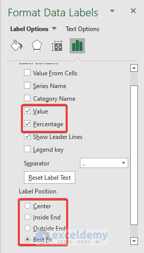
Our pie chart now displays both the percentage and value.

Read More: How to Show Total in Excel Pie Chart

Download Practice Workbook

Related Articles

• How to Create Pie Chart for Sum by Category in Excel
• How to Group Small Values in Excel Pie Chart
• How to Make Pie Chart by Count of Values in Excel
• How to Create Pie Chart Legend with Values in Excel

<< Go Back To Excel Pie Chart | Excel Charts | Learn Excel