How to Create Pie Chart Legend with Values in Excel

When we want to visualize the formation of a particular thing, we use the Pie Chart. For example, we can easily understand the business sales by region from the Pie Chart. In this article, we will show you 2 quick methods to create an Excel Pie Chart Legend with values.

How to Create Pie Chart Legend with Values in Excel: 2 Handy Approaches

To demonstrate our methods, we have selected a dataset with 2 columns: “Country” and “Sales”. Using these data, we will construct a Pie Chart in Excel. Basically, our dataset represents the sales values by country for a particular company.
Now, by default, the Legend does not show values beside it. Therefore, we need to follow some additional procedures to display the Legend with values.

1. Editing Horizontal Axis Labels to Create Excel Pie Chart Legend with Values

In this section, first, we create a basic Pie Chart with our data. Then, we will use the CONCATENATE function to join values into a single cell. After that, we copy those and “Paste as Values” into a single cell. Lastly, we input those values from the cell into the Horizontal Axis Labels, which will create an Excel Pie Chart Legend with values.

Steps:

To begin with, select the cell range B4:C9.
Next, from the Insert tab → Insert Pie or Doughnut Chart → select Pie.

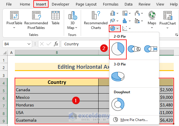
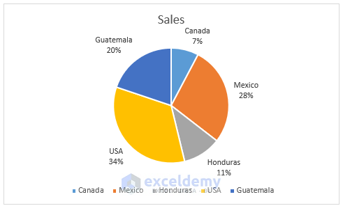
So, this basic Pie Chart will pop up. Moreover, notice there is Legend without values.

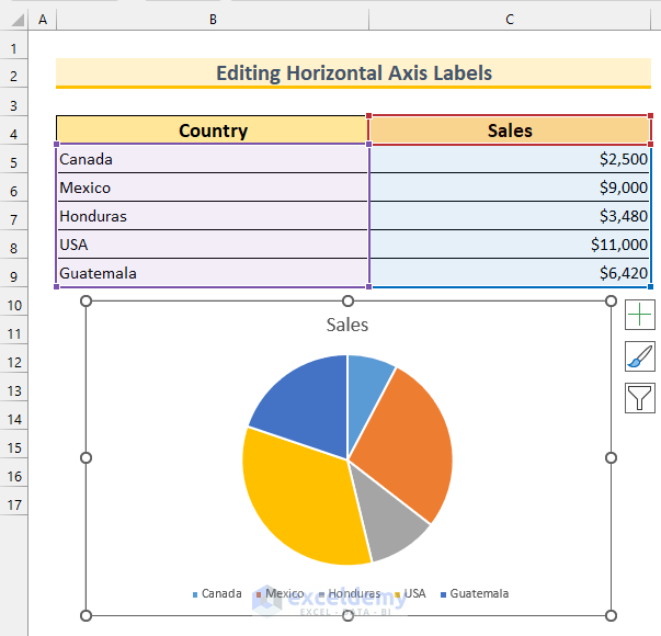
Next, we will add values to the Legend and modify the Pie Chart.
At first, we add Data Labels to the Pie Chart.
So, click on the Pie Chart and select Chart Elements.

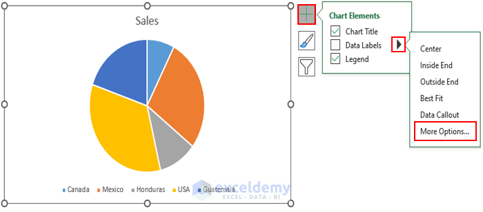
Then, the Format Data Labels box will appear.
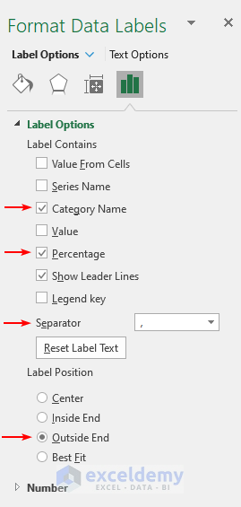
Then select these:
- Label Contains → “Category Name”, and “Percentage”.
- Separator → Comma.
- Label Position → Outside End.

Afterward, the Pie Chart will look like this.

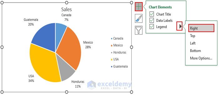
Secondly, we will move the Legend to the right side.
Hence, click on the Chart and select Chart Elements.
Then, select Right from the Legend option.
Therefore, our Legend will move to the right side.

Now, we will add values to the Pie Chart Legend.
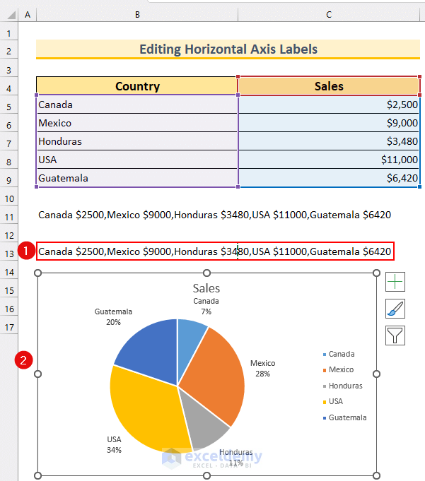
Firstly, type the following formula in cell B11.

=CONCATENATE(B5," ","$"&C5,",",B6," ","$"&C6,",",B7," ","$"&C7,",",B8," ","$"&C8,",",B9," ","$"&C9)

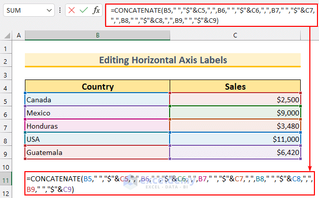
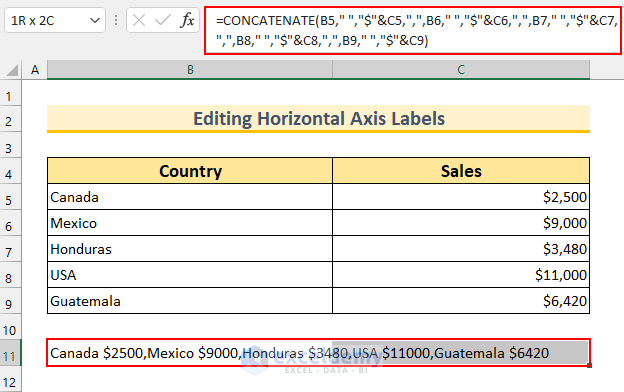
This formula joins the values with a single space and dollar signs. Thus, we will have all the values joined in a single cell.

Then, press ENTER.

Now, copy this value and “Paste as Values” in cell B13.

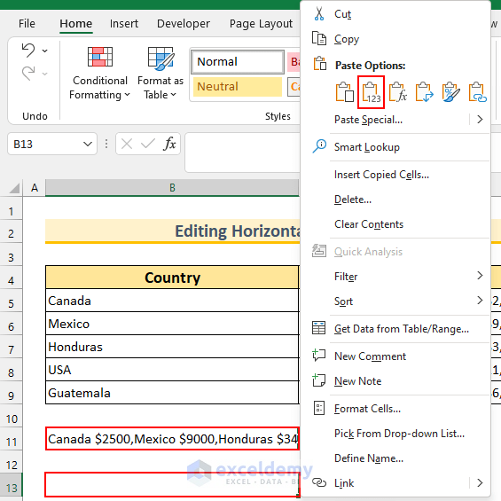
Then, copy the values from cell B13.
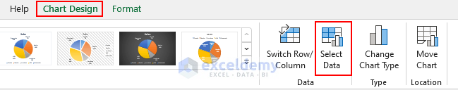
Afterward, select the Pie Chart.

Then, from the Chart Design tab, click on “Select Data”.

After that, the Select Data Source box will pop up.
Then, click on Edit under the “Horizontal (Category) Axis Labels” part.

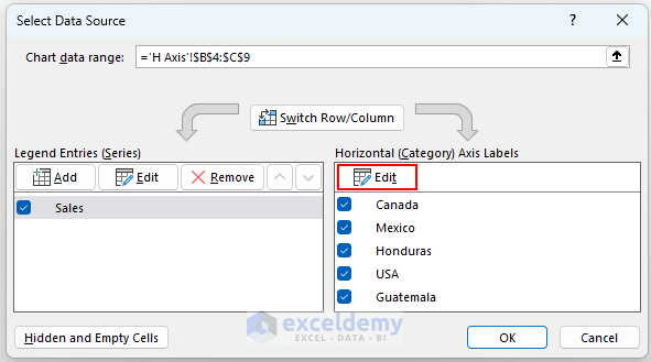
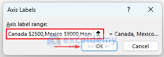
Next, another box will appear.
Afterward, paste the values inside the Axis label range.
Lastly, press OK twice.

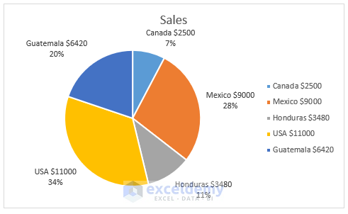
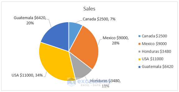
Thus, we will create an Excel Pie Chart Legend with values and this is what the final step should look like.

2. Using Combined Formula to Make Excel Pie Chart Legend with Values

For the last method, we will use the TEXT function along with the ampersand to create a formula to create the Legend. Then use these to make an Excel Pie Chart Legend that contains values.

Steps:

At first, select the cell range C5:C9 and type the following formula.

=B5&" " &TEXT(D5,"$0")

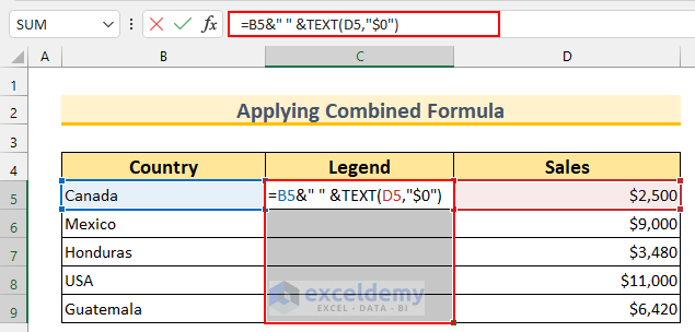
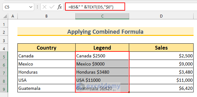
Then, press CTRL+ENTER.
This will AutoFill the formula to the selected cells.

Then, as shown in method 1, create the Pie Chart by selecting the cell range C4:D9.
Moreover, we have moved the Legend to the right side and added Data Labels to the Pie Chart.

Practice Section

We have added a practice dataset for each method in the Excel file. Therefore, you can follow along with our methods easily.

Download Practice Workbook

Pie Chart Legend.xlsx

Conclusion

We have shown you 2 handy approaches for creating a Pie Chart Legend with values in Excel. If you face any problems regarding these methods or have any feedback for me, feel free to comment below. Moreover, you can visit our site ExcelDemy for more Excel-related articles. Thanks for reading, keep excelling!

<< Go Back To Excel Pie Chart | Excel Charts | Learn Excel

Get FREE Advanced Excel Exercises with Solutions!