How to Create a Pie Chart by Count of Values in Excel (2 Methods)

Dataset Overview

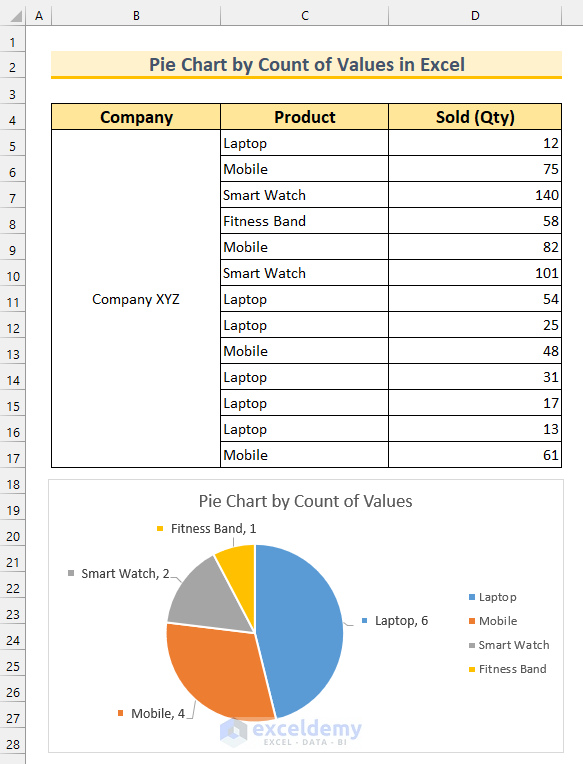
To illustrate the methods, we’ve chosen a dataset with three columns: Company, Product, and Sold (Qty).

Method 1 – Creating a Pie Chart Using Combined Functions

Unique Values:

• Format the cell range B19:C23.
• In cell B20, enter the formula:

• • This formula identifies unique values from the selected cell range.

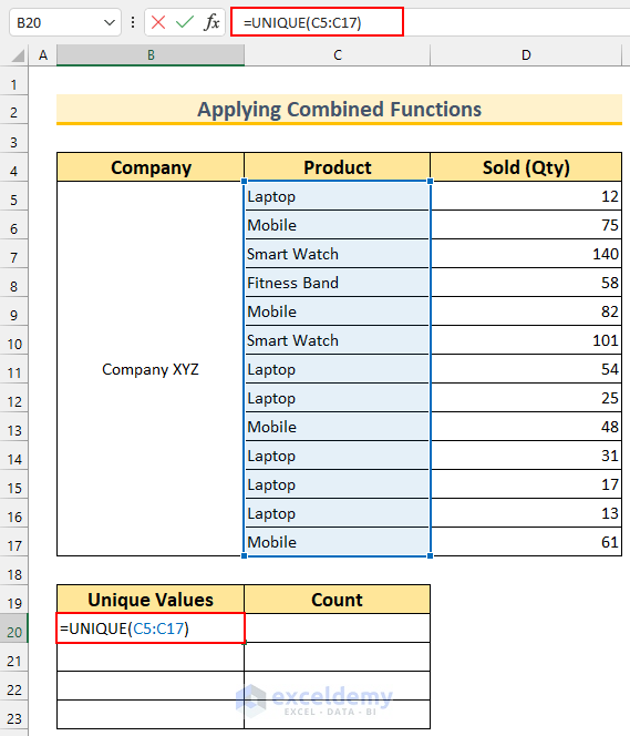
• Press ENTER.
• In the cell range C20:C23, enter:

• • This formula counts occurrences of unique values (using absolute cell references).

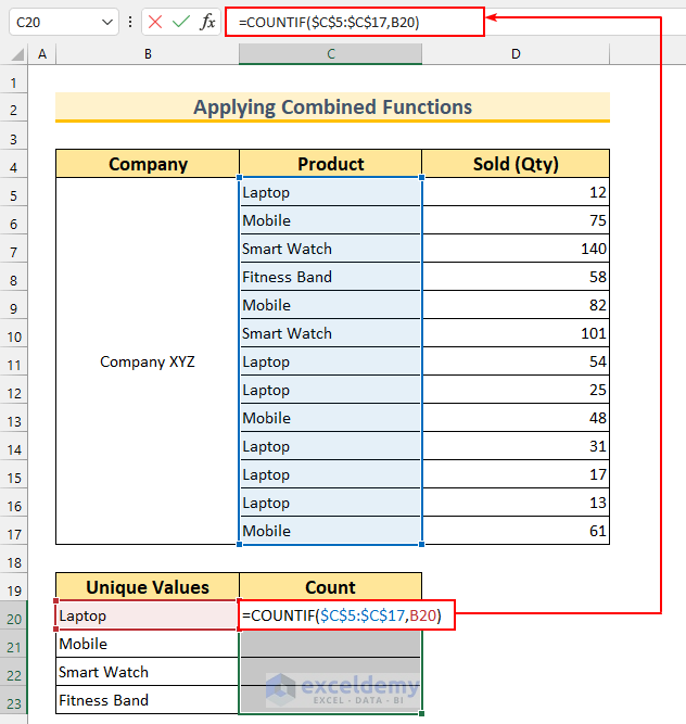
• Press CTRL+ENTER to autofill the formula.

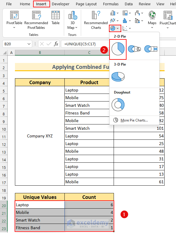
Inserting the Pie Chart:

• Select the cell range B20:C23.
• Go to the Insert tab, select Insert Pie or Doughnut Chart and choose Pie.

• Customize the chart by adjusting elements like the legend position and data labels.

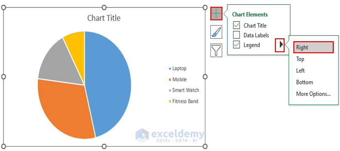
• Select the graph.
• From the Chart Elements, click on Legend and select Right. This will move the Legend to the right side of the graph.

• From the Data Labels, select “More Options…”.

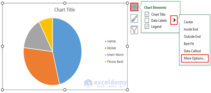
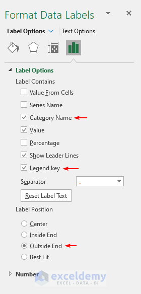
• The Format Data Labels box will appear on the right side of our Workbook.
• Select Category Name, and Legend Key from the Label Contains section.
• Select Outside End from the Label Position section.

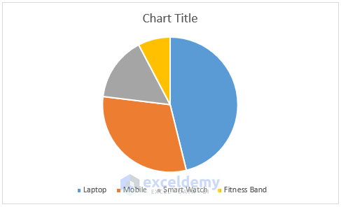
• By doing so, the Pie Chart will look like this.

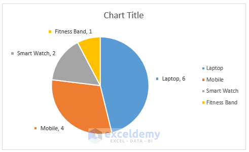
• We added a Chart Title, increased font size, and moved the Data Labels a bit to show the Leader Lines.
• The output represents our first method.

Read More: How to Show Percentage and Value in Excel Pie Chart

Method 2 – Creating a Pie Chart Using PivotTable

PivotTable Approach:

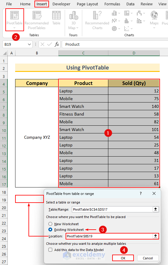
• Select the cell range C4:D17.
• From the Insert tab, choose PivotTable.
• Specify Existing Worksheet and cell B19 as the output location.
• Press OK.

• It brings a blank PivotTable.

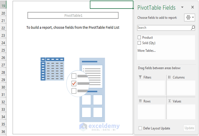
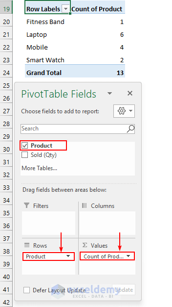
• Drag the Product field to Rows and Values in the PivotTable Fields window.
• The PivotTable displays unique values and their counts.

• Creating the Pie Chart:
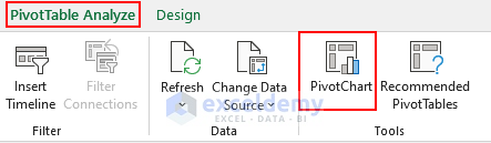
  • Select the PivotTable.
  • From the PivotTable Analyze tab, choose PivotChart.

• In the Insert Chart window, select Pie and confirm.

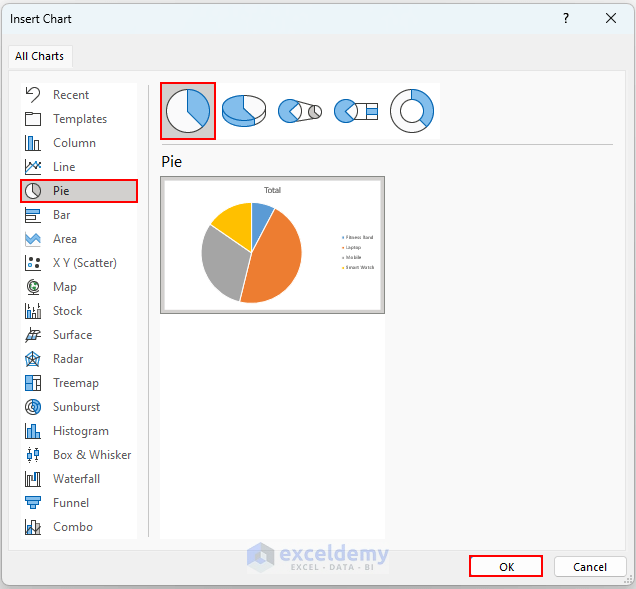
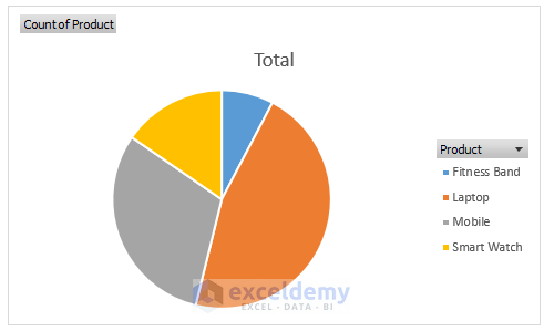
• The resulting basic Pie Chart shows value counts.

• Customize the chart as needed.

Read More: How to Show Percentage in Excel Pie Chart

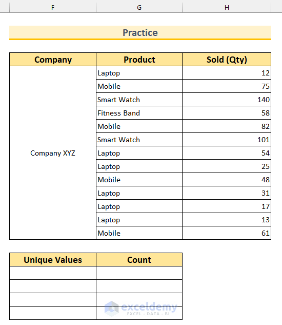
Practice Section

We have added a practice dataset for each method in the Excel file.

Download Practice Workbook

You can download the practice workbook from here:

Related Articles

• How to Show Percentage in Legend in Excel Pie Chart
• How to Show Total in Excel Pie Chart
• How to Create Pie Chart for Sum by Category in Excel
• How to Group Small Values in Excel Pie Chart
• [Solved]: Excel Pie Chart Not Grouping Data
• How to Create Pie Chart Legend with Values in Excel

<< Go Back To Excel Pie Chart | Excel Charts | Learn Excel