There are some built-in formats for phone numbers in Excel, so if you want to try other formats using the built-in formats, then, of course, it won’t work. But no worries! There is hope. I’ll introduce some tricky ways to overcome those situations if the phone number format is not working in Excel with clear steps and screenshots.
Excel Phone Number Format Not Working: 2 Possible Cases
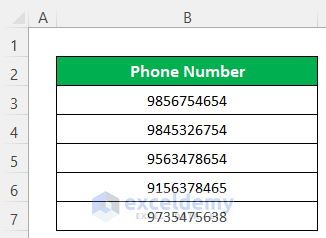
To demonstrate the methods, let’s use the following dataset that contains some random phone numbers. But it has no formatting. Now, we will see 4 cases, when you are unable to apply the built-in phone number format of Excel, or, the built-in feature is not what you want, so you need to customize the phone numbers.
Case 1: Excel Built-In Phone Number Format Is Not What You Want So Use a Custom Format
Have a look that there are no hyphens or brackets between the numbers. Let’s see what happens if we change the format to a custom phone number format.
Steps:
- Click on the Format Cells shortcut icon, as shown in the image below.
Soon after, a dialog box will open up.

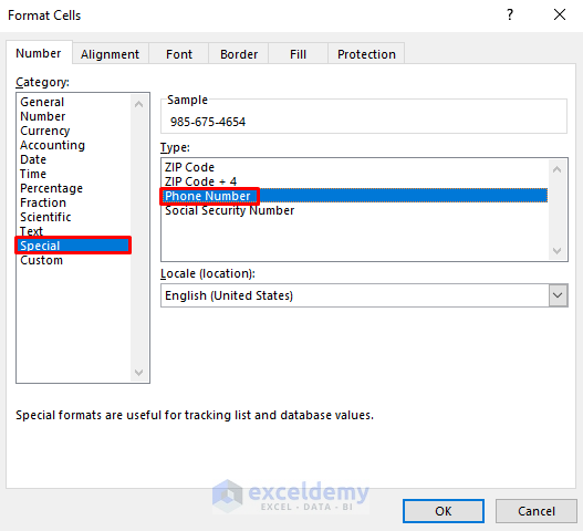
- Then click on Special from the Category section.
- Later, select Phone Number from the Type: section.

It’s the default phone number format in Excel.
But if you want to keep the format like this: XXX-XXX-XXXX, then that process won’t work.
Now let me show you how we can do it.
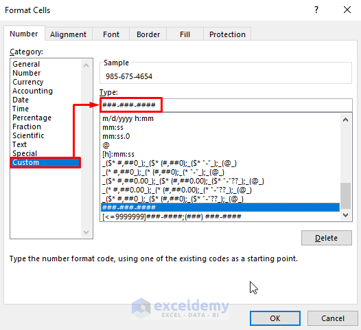
- Click on Custom from the Category section.
- Then type ###-###-#### in the Type: box.
- Finally, just press OK.
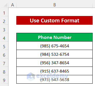
Now you see, our desired format worked well.

Read More: How to Format Phone Number with Dashes in Excel
Case 2: Your Numbers Have Hyphens in Them and Excel Rejects to Format Them as Phone Numbers
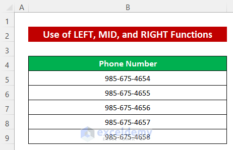
Let’s see another common issue. Here, the phone numbers are with hyphens.
Now, if we try the built-in Phone Number format, then see what it returns.
No change!
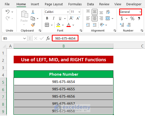
The reason the hyphens of the numbers were not returned with formatting is that they were typed in General format. Only the number format can be converted to the default phone number format.
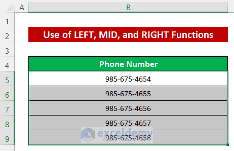
Solution 1: Apply a Formula with LEFT, MID and RIGHT Functions to Get Rid of Hyphens and Convert the Output to Number First
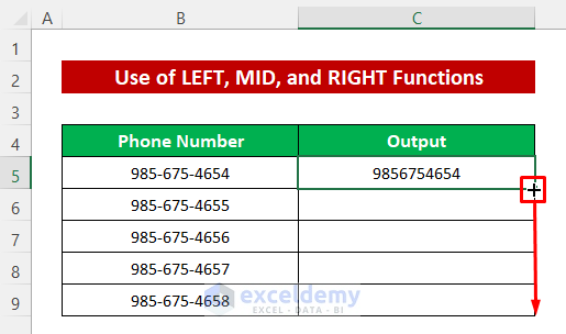
So, to get the numbers without hyphens, we’ll use the LEFT, MID, and RIGHT functions. For that, I added a new column.
Steps:
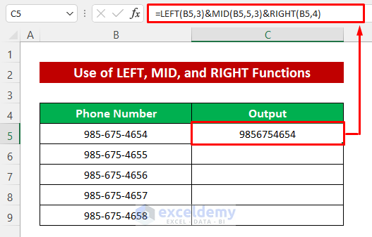
- Write the formula in Cell C5–
=LEFT(B6,3)&MID(B6,5,3)&RIGHT(B6,4)Later, just press the Enter button and see that all the hyphens are removed.
- Finally, drag down the Fill Handle icon to copy the formula for the other cells.
Then, you will get all the numbers without hyphens.

Now, we’ll have to convert the values into numbers. For that, I have added a new column.
- Copy the outputs and.
- Then select the first cell of the new column.
- Later, right-click your mouse and paste them as values.

The values are stored as text here.
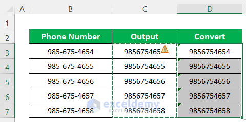
- Click on the error icon and select Convert to Number.

Now see that the error message is gone and converted to numbers.
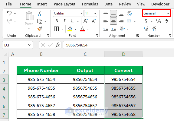
Now you can change the format to a special Phone Number format.

We are done.

🔻 Formula Breakdown:
➽ LEFT(B5,3)
The LEFT function will return the first three digits from the number of Cell B5–
“985”
➽ MID(B5,5,3)
The MID function will keep three digits starting from the fifth position of the number so that it will return as
“675”
➽ RIGHT(B5,4)
The RIGHT function will return the last four digits from the number of Cell B5–
“4654”
➽ LEFT(B5,3)&MID(B5,5,3)&RIGHT(B5,4)
Finally, the & operator will join the outputs together, and that will return as
“9856754654”
Read More: Excel Formula to Change Phone Number Format
Solution 2: Apply SUBSTITUTE Function to Get Rid of Hyphens
You can remove the hyphens using the SUBSTITUTE function, too. It’s fast and easy compared to the previous method.
Steps:
- In Cell C5, type the following formula-
=SUBSTITUTE(B5,"-","")- Then press the Enter button.
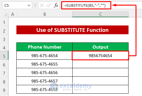
- Finally, use the Fill Handle tool to finish.
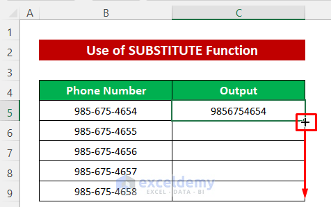
And we get all the numbers without hyphens.

Now, we’ll have to convert the values into numbers. For that, I have added a new column.
- Copy the result.
- Now, select the first cell of the new column.
- Right-click your mouse and paste them as values.
The values are in text format here.
- To convert them to number format, click on the error icon and select Convert to Number.
Now see that the error message is gone and converted to numbers.
Now, you can change the format to a built-in Phone Number format.
Here is the final result!
Read More: How to Remove Parentheses from Phone Numbers in Excel
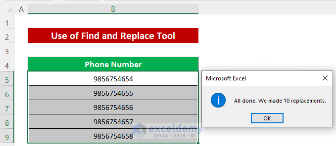
Solution 3: Use the Find and Replace Tool to Replace the Hyphens
Here, we’ll use the Find and Replace tool if the phone number formats of Excel don’t work. We can easily remove all the hyphens at a time from numbers using this tool.
Steps:
- Select the cells that contain numbers.
- Press Ctrl+H to open the Find and Replace dialog box.
- Then type a hyphen (-) in the Find what: box and keep the Replace with: box empty.
- Finally, just press Replace All.

Soon after, you will see that the tool has removed all the hyphens successfully.
Now, we’ll convert these into numbers. For that, execute the following steps.
- Copy the outputs.
- Then select the first cell of the new column.
- Later, right-click your mouse and paste them as values.
The values are stored as text here.
- Click on the error icon and select Convert to Number.
Now see that the error message is gone and converted to numbers.
Now you can change the format to a special Phone Number format.
Thus, we have successfully fixed the issue.
Download Practice Workbook
You can download the free Excel template from here and practice on your own.
Conclusion
I hope the procedures described above will be good enough to solve the problem if the phone number format is not working in Excel. Feel free to ask any questions in the comment section, and please give me feedback.
Related Articles
- How to Write Phone Number in Excel
- Keep 0 Before a Phone Number in Excel
- How to Format Phone Number with Country Code in Excel
- How to Format Phone Number with Extension in Excel
<< Go Back to Phone Number Format | Number Format | Learn Excel
Get FREE Advanced Excel Exercises with Solutions!

