An Excel Formula to Change the Phone Number Format

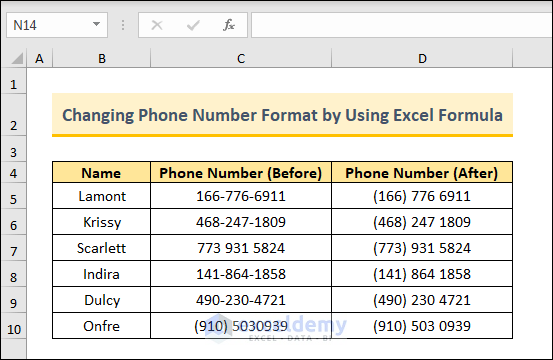
The dataset showcases phone numbers before and after changing their formatting.

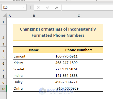
Changing Inconsistently Formatted Phone Numbers to a Specific Format

The dataset contains phone numbers with no uniform formatting.

Method 1 – Combining SUBSTITUTE & TEXT Functions

Use the SUBSTITUTE function and the TEXT function to change the phone number format.

The SUBSTITUTE function removes unnecessary characters (dashes, commas, blanks etc) and makes them plain numbers. The TEXT function formats the plain number.

• Select a blank cell and enter the following formula:
  =TEXT(SUBSTITUTE(SUBSTITUTE(SUBSTITUTE(SUBSTITUTE(C5,")",""),"(","")," ",""),"-",""), "(###) ### ####")
• Click Enter.
  The phone number will change to the (###) ### #### format.
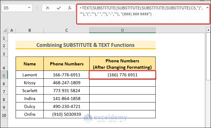  All dashes were replaced with spaces and the code area (first three digits) were enclosed using parentheses.

• Use the Fill Handle to fill the rest of the cells.
  

This is the output.

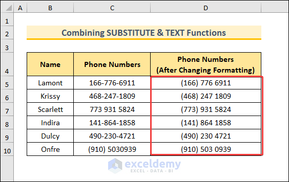
The SUBSTITUTE function was used four times to replace non-number symbols like commas, spaces, and parentheses. Add more SUBSTITUTE functions to the formula if there are more non-number symbols.

You can change the formatting code “(###) ### ####” in the argument of the TEXT Function.

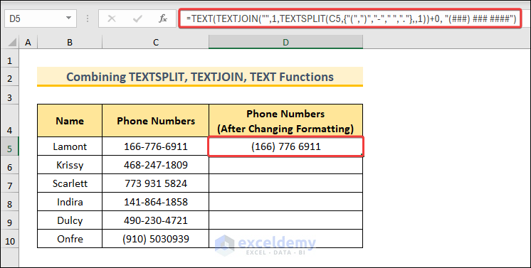
Method 2 -Combining the TEXTSPLIT, TEXTJOIN, and TEXT Functions

Combine the TEXTSPLIT, TEXTJOIN, and TEXT functions:

• Select a blank cell and enter the following formula:
  =TEXT(TEXTJOIN("",1,TEXTSPLIT(C5,{"(",")","-"," ","."},,1))+0, "(###) ### ####")
• Press Enter.
  
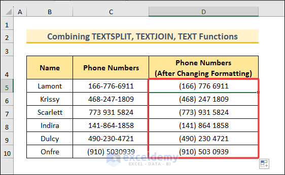
• Use the Fill Handle to copy the formula to the rest of the cells.

Phone numbers changed to a common format.

In the formula, the TEXTSPLIT function splits text using specified delimiters such as parentheses, hyphens, spaces, and dots. You can group all delimiters in a single array  {“(“,”)”,”-“,” “,”.”} and use it in the argument, which also removes the delimiters. The split texts are then joined using the TEXTJOIN function. 0 is added to convert it into a numeric value. The resultant numeric values are formatted as phone numbers using the TEXT function.

Note: Converting the rejoined texts into a numeric value, removes the leading zeros from phone numbers.

Read More: [Solved!]: Excel Phone Number Format Not Working

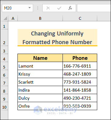
Changing a Formatted Phone Number to a Specific Format

The dataset contains a list of phone numbers with the same formatting.

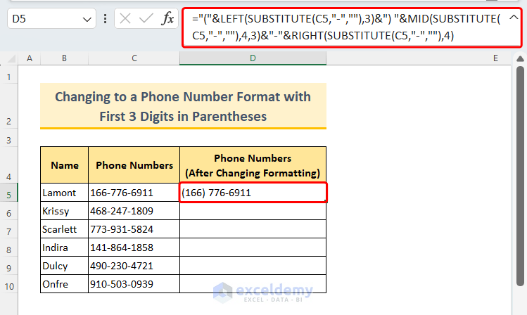
Example 1- Changing to a Phone Number Format with the First 3 Digits in Parentheses

Combine the LEFT, MID, RIGHT, and SUBSTITUTE functions.

• Select a blank cell and enter the following formula:
  ="("&LEFT(SUBSTITUTE(C5,"-",""),3)&")"&MID(SUBSTITUTE(C5,"-",""),4,3)&"-"&RIGHT(SUBSTITUTE(C5,"-",""),4)
  
• Press Enter to see the result.
  
• Use the Fill Handle to fill the rest of the cells.

All phone numbers will change.

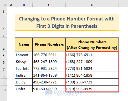
In the formula, the SUBSTITUTE function removes hyphens from the original number. The LEFT function extracts the first three digits, which are enclosed within parentheses. The MID function extracts the next three digits. The RIGHT function extracts the last four digits.

Note:  This formula is only applicable to 10 digit phone numbers with hyphens in 4th and 8th place as delimiters.

Read More: How to Remove Parentheses from Phone Numbers in Excel

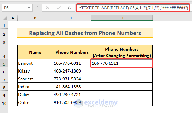
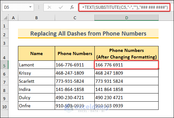
Example 2: Replacing All Dashes in Phone Numbers

Use the REPLACE and the TEXT functions.

• Select a blank cell and use the following formula:
  =TEXT(REPLACE(REPLACE(C5,4,1,""),7,1,""),"### ### ####")
  
• Press Enter to see the result.
  
• Use the Fill Handle to fill the rest of the cells.

All phone numbers will change.

In the formula, the innermost REPLACE function eliminates the dash in the 4th position and the result is transferred into the outer REPLACE function. The outer function removes the dash in the 7th position. The result is formatted using the TEXT function with the pattern “### ### ####”.

Note: If you have dashes occurring more than twice, use the SUBSTITUTE function to eliminate all dashes:

=TEXT(SUBSTITUTE(C5,"-",""),"### ### ####")

Read More: How to Format Phone Number with Dashes in Excel

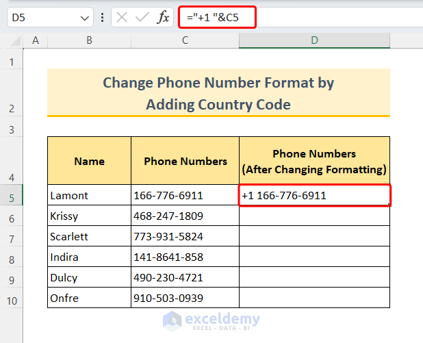
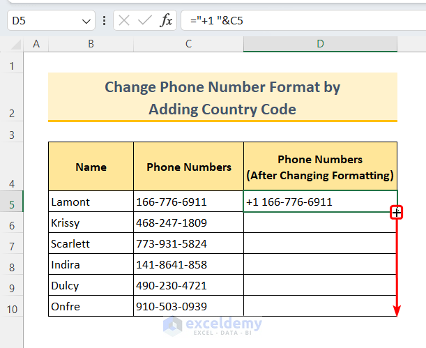
Example 3 – Changing the Phone Number Format by Adding the Country Code

Use the Ampersand (&) operator to add the country code to phone numbers in Excel.

• Use the following formula in a blank cell:
  ="+1 "&C5
• Press ENTER.
  The first phone number is formatted .
  
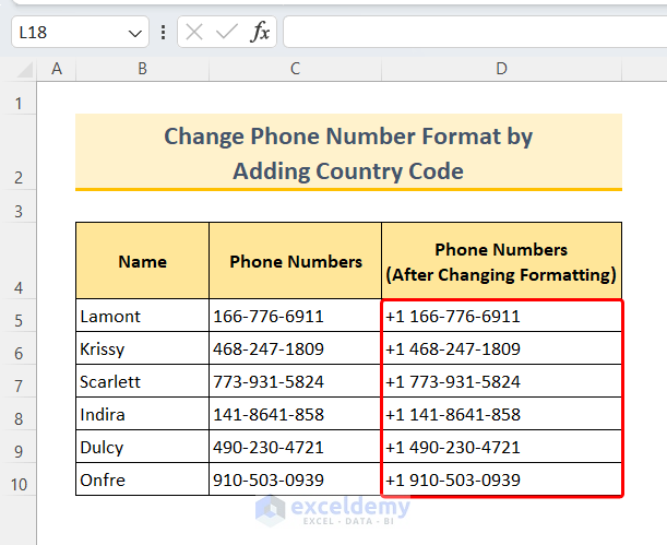
• Autofill the formula using the Fill Handle.
  

The country code will be added to the phone numbers.

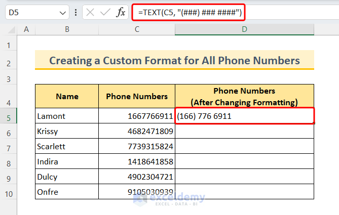
Example 4 – Creating a Custom Format for All Phone Numbers

Use the TEXT function.

• Select a blank cell and enter the following formula:
  =TEXT(C5, "(###) ### ####")
  
• Press Enter to see the result.
  
• Use the Fill Handle to autofill the rest of the cells.

This is the output.

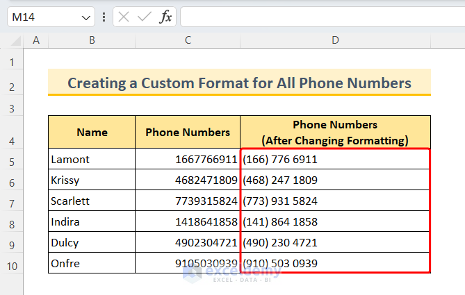The format code takes the first three digits as area codes and encloses them inside parentheses. There will be spaces in the 4th and 8th places.

Note: This formula will not work for a mixed format of phone numbers.

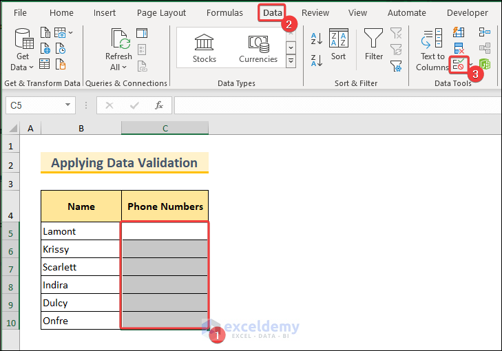
How to Ensure a Uniform Phone Number Entry Using Data Validation

Use the Data Validation tool.

• Select the range of cells to apply data validation.
• Go to the Data tab > Data Tools > Data Validation.
  

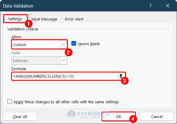
In the Data Validation dialog box:

• Go to Settings.
• In Allow, choose Custom.
• In Formula, enter the following formula:
  =AND(ISNUMBER(C5),LEN(C5)=10)
• Click OK.

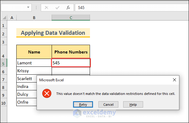
An error message will be displayed if you enter values, other than a 10-digit number.

Download Practice Workbook

Download the practice workbook.

Frequently Asked Questions

How Do I Add a Dash Between Phone Numbers in Excel?

Use the following formula:
=TEXT(A1,”000-000-0000″)
Replace A1 with the cell containing the phone number in plain number format and customize the format code “000-000-0000” to match the specific number of digits in the phone number. Adjust the dash positions.

Are There Built-In Phone Number Formats For Phone Numbers In Excel?

Yes, there are built-in phone number formats in Excel which you can access in the Format Cells dialog box:

1. Select the cells that contain phone numbers
2. Press Ctrl+1 to open the Format Cells dialog box.
3. In the Format Cells dialog box:
   • Go to the Number tab;
   • In Category, click Special;
   • In Locale(location), select your location;
     The available format types for the location will be displayed in Type;
   • In Type, select a format;
     You can preview different types in “Sample“.
   • Click OK.

Related Articles

• How to Write Phone Number in Excel
• Keep 0 Before a Phone Number in Excel
• How to Format Phone Number with Extension in Excel

<< Go Back to Phone Number Format | Number Format | Learn Excel