How to Format Phone Number with Dashes in Excel: 2 Methods

Method 1 – Using Format Cells Option

1.1 Using Special Category

Excel has some built-in number formats which you can access from the Format Cells window. Among the options in the Special category, there is also a Phone Number format which you can use to format your phone numbers with dashes.

To use the Special category in the Format Cells dialog box to format phone numbers with dashes, follow the steps below:

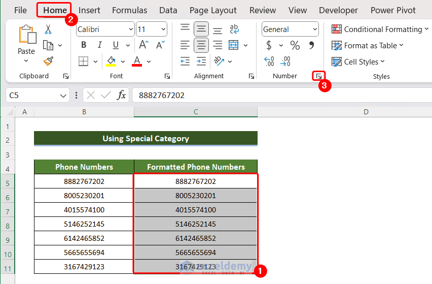
1. Select the cells containing phone numbers that you want to format.
2. Go to the Home tab > Number group > Dialog Box Launcher.
   Click on the Ctrl+1 shortcut key to open the Format Cells dialog box.
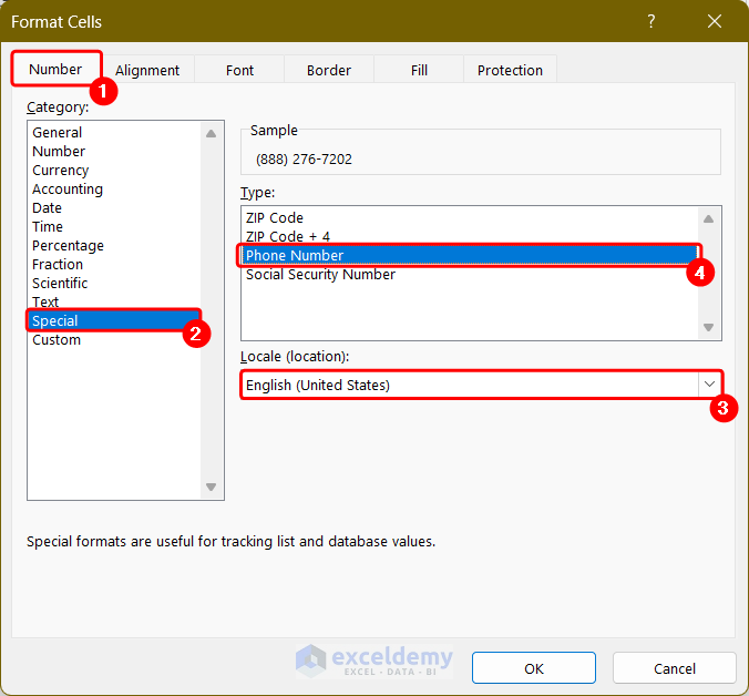
   The Format Cells dialog box will appear.
3. In the Format Cells dialog box:
   • Go to the Number tab;
   • Under Category, click Special;
   • Under the Locale(location), select your location from the available drop-down options;
     The available format types for that location will be displayed under the Type menu;
   • Under the Type, select the format that has dashes;
     Preview them under “Sample” to help you choose.
   • Press OK.

   

The phone numbers will be formatted according to your chosen format.

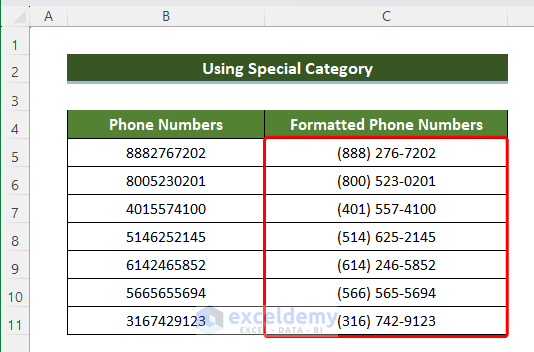
We chose English (United States) as the Locale(location) and Phone Number as the format type. The first three digits which denote the area code are enclosed by parentheses, and the rest of the digits are separated by a dash. You need to select the parameters accordingly.

1.2 Using Custom Number Format

If you don’t find your Locale(location) or the desired special format in the Format Cells dialog box, you can create your own custom format.

To use the custom format to format phone numbers with dashes, follow the steps below:

1. Select the range of cells that contain phone numbers that you want to format.
2. Press Ctrl+1 to open the Format Cells dialog box.
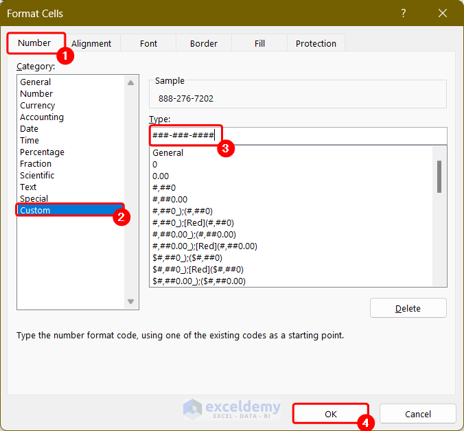
3. In the Format Cells dialog box:
   • Go to the Number tab;
   • Under Category, click Custom;
   • In the Type field, write the following number format code:
     ###-###-####
Here, each # represents a digit. So adjust the number of # according to your phone number’s digits.
   • Press OK.

   

The phone numbers will be formatted with dashes.

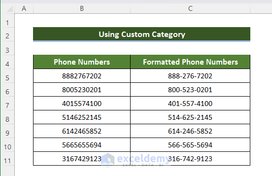
A good thing about using this method is that only the appearance of the phone numbers changes, but the values of the phone numbers remain unaltered. You can select any formatted cell and see the value in the formula box.

Method 2 – Using Excel Functions

We can also format the phone numbers using various types of formulas like REPLACE, TEXT, and different types of string functions like LEFT, LEN, RIGHT, MID, etc. The formulas keep the original numbers intact and store the formatted phone numbers in a new location. All these methods are explained with examples below.

2.1 Using Replace Function

The REPLACE function replaces part of a text string, based on the number of characters you specify, with a different text string.

To format phone numbers with dashes using the REPLACE function, follow the steps below:

1. Select a blank cell and enter the following formula:
   =REPLACE(REPLACE(B5,4,0,"-"),8,0,"-")
   Cell B5 indicates the first cell of the dataset containing the phone number. Replace cell B5 with your dataset’s first cell.
2. Press Enter.
   The destination cell will contain the formatted number with a dash.
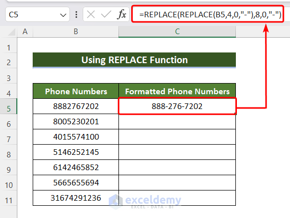   We wanted to insert two dashes after the 3rd and 6th character; in the formula, the inner REPLACE function adds a dash after the 3rd character by starting at the 4th position, and the outer REPLACE function, building on the modified text, adds another dash after the 6th character by starting at the 8th position.
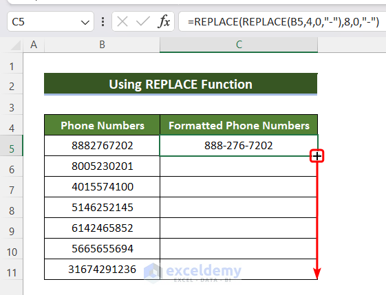
3.  Use the Fill handle icon in the corner of the cell and drag it down to the end of the dataset.
   

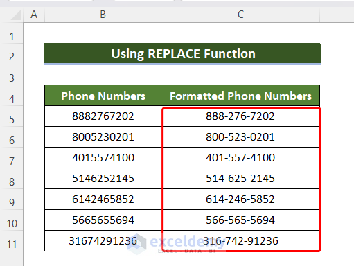
All the phone numbers will be formatted with dashes.

Note: In this formula, if you wish to include additional dashes, you can achieve that by adding more instances of the REPLACE function. If you want to adjust the positions where the dashes are inserted, modify the second argument within each REPLACE function. The second argument determines the starting position for inserting the dashes.

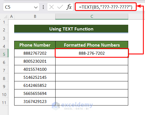
2.2 Using TEXT Function

The TEXT function, users can specify in which format the content of a cell will be displayed. You can also use it to format phone numbers with dashes.

Know how to format phone numbers with dashes with the help of the TEXT function, follow the steps below:

1. Select a blank cell and write the following formula
   =TEXT(B5,"???-???-????")
Replace B5 with the first cell of the unformatted phone number column.
2. Press the ENTER button.
   You will see a formatted phone number.
   
3. Drag the Fill Handle button in the corner of the cell down to the end of the dataset.

All the phone numbers will be formatted with dashes like this.

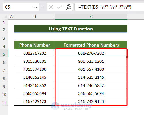
Note: In the 2nd argument of the TEXT function, each “?” represents a character. Here, you can add more “?” or adjust the position of the dashes according to the phone numbers of your dataset.

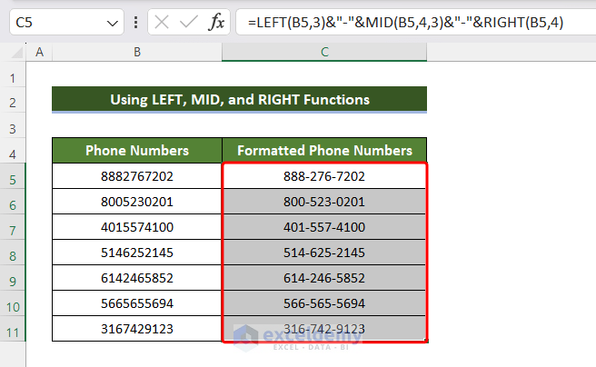
2.3 Using LEFT, MID, and RIGHT Functions

By using various string functions like LEFT, MID, and RIGHT, the users can extract certain parts of a text and piece them together with the help of the Ampersand operator (&) after inserting dashes in the desired positions.

How to use the LEFT, MID, and RIGHT functions to format phone numbers with dashes in Excel, follow the steps below:

1. Select a blank cell and write the following formula
   =LEFT(B5,3)&"-"&MID(B5,4,3)&"-"&RIGHT(B5,4)
Replace B5 with the first cell of the unformatted phone number column.
2. Press the ENTER button.
   You will see a formatted phone number.
   In the formula, the LEFT(B5,3) extracts the first three characters, followed by a dash, then MID(B5,4,3) extracts the middle three characters starting from the 4th position with another dash, and finally, RIGHT(B5,4) captures the last four characters.
3. Dag the Fill Handle button in the corner of the cell down to the end of the dataset.

All the phone numbers will be formatted with dashes like this.

Note: The formula that I provided above works only for 10-digit numbers and it only adds dashes after the 3rd and 6th character. You need to change them accordingly. For example, If you have 12 digits phone number and you want to format it in ###-####-##### format, you need to modify the formula in the following way:
=LEFT(B5,3)&"-"&MID(B5,4,4)&"-"&RIGHT(B5,5)

Download Practice Workbook

Download this practice workbook from the link below.

.

Frequently Asked Questions

What Is the Advantage of Using Format Cells Over Formulas?

Using Format Cells directly modifies the visual appearance of phone numbers without requiring additional cells for storage. It offers a convenient way to customize formats while keeping the original values intact.

How Do I Revert to the Original Phone Number Format After Formatting With Dashes?

If you’ve used the Format Cells option, you can easily revert to the original format by selecting the cells, right-clicking, choosing “Format Cells,” and selecting “General” under the Number tab.

Related Articles

• How to Format Phone Number with Country Code in Excel
• How to Format Phone Number with Extension in Excel
• Keep 0 Before a Phone Number in Excel
• [Solved!]: Excel Phone Number Format Not Working

<< Go Back to Phone Number Format | Number Format | Learn Excel