How to Use NOT and ISNA Functions in Excel (2 Examples)

Get FREE Advanced Excel Exercises with Solutions!

The tool known as Microsoft Excel is quite helpful. You can execute an infinite number of operations on a dataset using Excel‘s tools and capabilities. When working with Excel, we frequently need to employ a combination of NOT and ISNA statements. Nevertheless, combining NOT and ISNA functions is necessary for many scenarios. This article looks at two scenarios suited for putting the combination of NOT and ISNA functions into practice. As a result, you should be bold and walk through these two real-world examples to learn how to utilize the NOT and ISNA functions in Excel.

Table of Contents hide

Download Practice Workbook

Why Do We Use NOT Function?

Why Do We Use ISNA Function?

2 Suitable Examples to Use NOT and ISNA Functions in Excel

1. Merge IF, NOT and ISNA Functions to Determine Not Available Type Error (#N/A) in Excel

2. Combine IF, NOT, VLOOKUP, and ISNA Functions to Search Items in Excel

Conclusion

Download Practice Workbook

If you would like a free copy of the illustrated workbook that we covered during the presentation, please click on the link that can be found just below this section.

NOT and ISNA Functions.xlsx

Why Do We Use NOT Function?

The NOT function gives the opposite result of the rational or Boolean answer sent into it. You can utilize the NOT function to get the opposite of a Boolean expression or the conclusion of a logical statement. Said it will always give the opposite of the expected logical value. The function assists in determining whether or not two values are equivalent to each other.

Why Do We Use ISNA Function?

In Excel, you can use the ISNA function to examine cells or formulae for mistakes involving #N/A notation. The outcome is a rational value, which is true (TRUE) when a #N/A mistake is found and false (FALSE) otherwise. Excel 365, as well as every previous version, all the way back to Excel 2000, have the feature in some form or another. Excel‘s ISNA function may be found under the Error handling functions. The ISNA function is fantastic since you can simultaneously organize both categories by the Check columns. The #N/A rows will be grouped and appear at the top, including both lists.

2 Suitable Examples to Use NOT and ISNA Functions in Excel

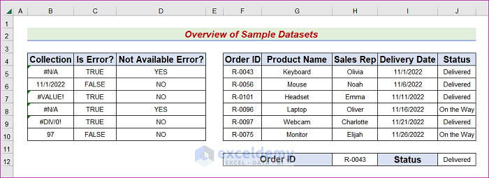
To illustrate this point, let’s examine two representative datasets. The first dataset consists of three columns: Collection, IS Error ?, and Not Available Error?. Using the combination of IF, NOT, and ISNA, we will create a formula to determine whether a cell contains a Not Available Type Error. In contrast, the second dataset has five columns: Order ID, Product Name, Sales Rep, Delivery Date, and Target Sales. Moreover, there is a search box titled Order ID, and the Status info box will display whether the order is complete. Both of these boxes belong to the second dataset. We will develop a combined formula using the IF, NOT, VLOOKUP, and ISNA functions to establish a system that takes a search item and display the order status.

Notes

I’ve also been using Microsoft Excel 365 to compose this post. You are free to select the version that best meets your needs, and whichever option you choose is acceptable to us.

1. Merge IF, NOT and ISNA Functions to Determine Not Available Type Error (#N/A) in Excel

Using the IF function, you can make inferences about a value based on whether or not it matches your expectations. If you pass a value to the NOT function, it will return the opposite value. We may use the ISNA function to determine if any given cell has the #N/A Error. These functions will be used in this context to check for the Not Available Error (#N/A) in a given cell. The nested procedure can help you get things done, so here are some steps.

STEPS:

Firstly, choose the intended sheet as the Active sheet.
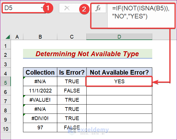
Second, select the D5 cell.
Third, input the below equation in the Formula bar.

=IF(NOT(ISNA(B5)),"NO","YES")

After that, hit the Enter or Tab key.
Subsequently, the result will display in D5.

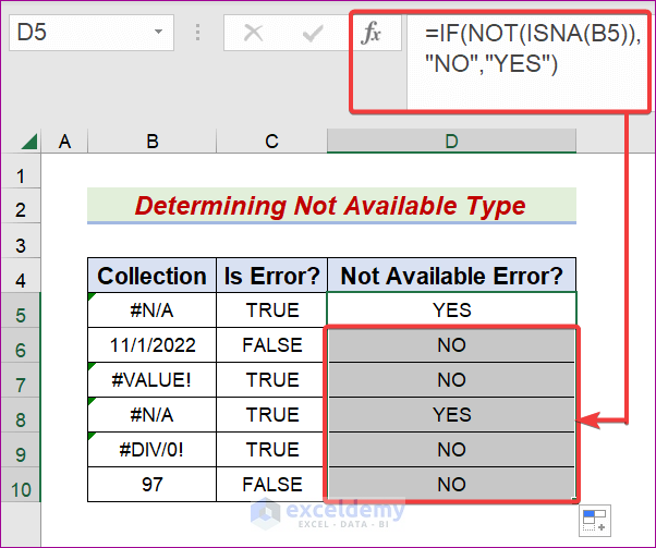
Now, we have to use the same formula in the other cells.
To achieve this, utilize the AutoFill Handle icon and drag it to cell D10.
As a result, it will produce the desired output like the below one.

Formula Breakdown

=IF(NOT(ISNA(B5)),"NO","YES")

To understand this formula, you must be familiar with the following Excel functions:

IF, NOT and ISNA Functions

ISNA(B5)

In this demonstration, by involving the ISNA function in the combination, we find TRUE.

NOT(ISNA(B5))

The NOT function will receive the output from the ISNA function and returns an opposite value. Here we will get FALSE from the NOT function.

IF(NOT(ISNA(B5)),”NO”,”YES”)

The IF function performs a logical evaluation and returns one value for a TRUE conclusion and another for a FALSE one. Here, the IF function will evaluate FALSE because of the output of the NOT function. Utilizing the IF function, we get YES.

2. Combine IF, NOT, VLOOKUP, and ISNA Functions to Search Items in Excel

The VLOOKUP function in Excel allows users to quickly and easily find matching records in an extensive data collection or table. Throughout this section, we will merge the IF, NOT, VLOOKUP, and ISNA functions together and build a formula that will be able to search for an item from a range. To complete the work with the assistance of the nested procedure, adhere to the guidelines below.

STEPS:

Firstly, choose the intended sheet as the Active sheet.
Second, select the D12 cell.
Third, input the desired Order ID.

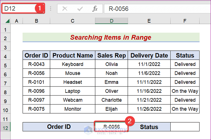
Likewise, pick the F12 cell.
After that, input the below equation in the Formula bar.

=IF(NOT(ISNA(VLOOKUP(D12,B4:F10,5,FALSE))),VLOOKUP(D12,B4:F10,5,FALSE),"Not Found")

Later, hit Enter.
Consequently, we will get the result like the following.

Formula Breakdown

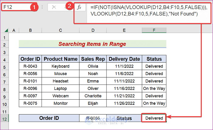
=IF(NOT(ISNA(VLOOKUP(D12,B4:F10,5,FALSE))),VLOOKUP(D12,B4:F10,5,FALSE),"Not Found")

For this formula to make sense, you need to know how to use the following Excel functions:

IF, NOT, VLOOKUP and ISNA Functions

VLOOKUP(D12,B4:F10,5,FALSE)

To search for a value in a table or range by its row number, we use the VLOOKUP function. In this demonstration, by involving the ISERROR function in the combination, we find Delivered.

ISNA(VLOOKUP(D12,B4:F10,5,FALSE))

Here, the ISNA function will produce FALSE because the output of the VLOOKUP function is not #N/A.

NOT(ISNA(VLOOKUP(D12,B4:F10,5,FALSE)))

In this demonstration, by involving the NOTfunction in the combination, we find TRUE.

IF(NOT(ISNA(VLOOKUP(D12,B4:F10,5,FALSE))),VLOOKUP(D12,B4:F10,5,FALSE),”Not Found”)

The IF function performs a logical evaluation and returns one value for a TRUE conclusion and another for a FALSE one. Utilizing the IF function, we get Delivered.

Conclusion

After this point, you can utilize the NOT and ISNA Functions in Excel by following the examples we discussed. On the ExcelDemy Website, you can discover numerous articles that are comparable to this one. Keep using them, and let us know if you have any other ideas or ways to accomplish the task or if you’re looking for something different to try. If you have any questions or comments, please submit them in the area below.