We often have to compare two rows or two columns in an Excel workbook. But if we do it without applying direct formulas, it becomes very tiresome. Excel helps us provide some functions to perform it easily. In this article, we’ll show you how Excel ISNA and MATCH functions make the work easy for us. We have used Microsoft 365 to do all the tasks.
How to Use ISNA Function with MATCH Function in Excel: 2 Suitable Examples
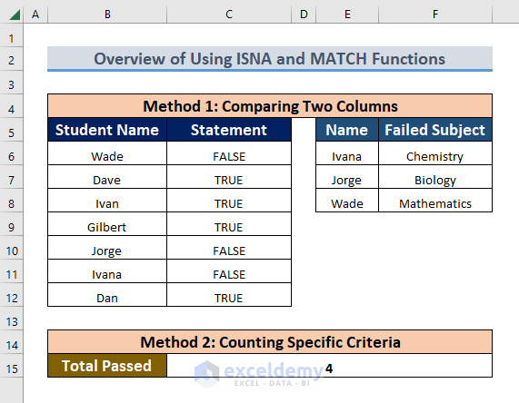
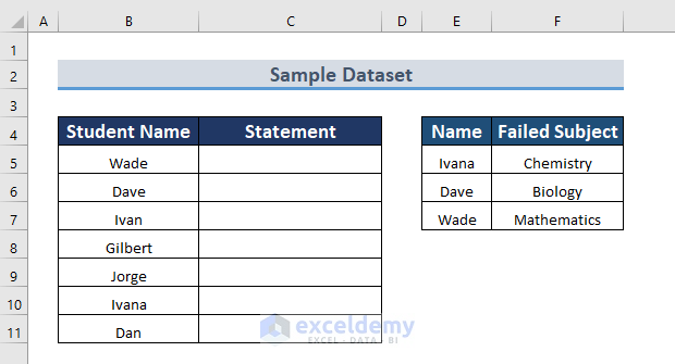
To illustrate, we will use a sample dataset. For instance, the following dataset comprises all the students’ names in a class as well as the students who failed in a subject.
1. Combining ISNA and MATCH Functions to Compare Two Columns in Excel
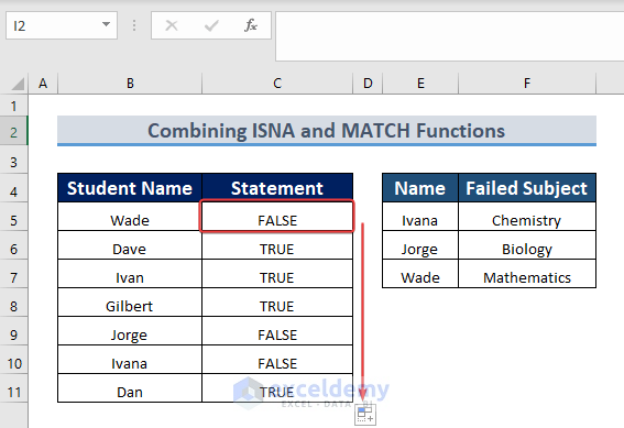
ISNA and MATCH functions are combined in the following example in order to compare columns. Column B contains all the students and compares with column E who failed and shows the value either a student passed or failed in the logic of TRUE or FALSE.
Steps:
- At first, we apply the following Formula in the C5 cell.
=ISNA(MATCH(B5,$E$5:$E$7,0))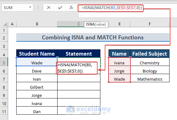
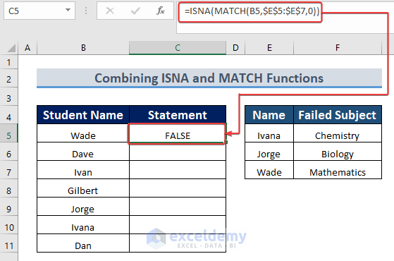
- So, if we hit ENTER on C5, we get a value in the C5 cell.
- After that, a plus sign appears in the lower corner of the cell.
- Finally, we will drag it down with the AutoFill feature to fill the remaining cells.
Formula Breakdown
- MATCH(B5,$E$5:$E$7,0) returns value 3 which implies it finds 3 matches with column B and column E.
- ISNA function takes the value returned by MATCH(B5,$E$5:$E$7,0) which is “3” as an argument and gives the result.
Read More: How to Use IF with ISNA Function in Excel
2. Merging ISNA, MATCH, and SUMPRODUCT Functions for Counting Specific Criteria in Excel
The unique 3 functions ISNA, MATCH, and SUMPRODUCT combinedly help us find specific criteria and the total number of that criteria. Suppose we want to find the total number of failed students and keep that value in another cell. We followed the following steps to do that.
Steps:
- Firstly, enter the formula in cell C13.
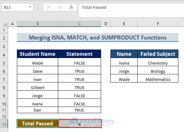
=SUMPRODUCT(--ISNA(MATCH($B$5:$B$11, $E$5:$E$7, 0)))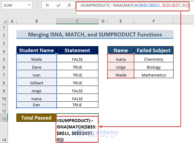
- After pressing ENTER, the data set will give the counted value.
Formula Breakdown
- MATCH($B$5:$B$11, $E$5:$E$7, 0) returns the number of matches between column B and column E.
- ISNAMATCH($B$5:$B$11, $E$5:$E$7, 0)) returns an array of TRUE FALSE.
- SUMPRODUCT takes the array of TRUE FALSE returned by ISNA(MATCH($B$5:$B$11, $E$5:$E$7, 0)) and returns the total count.
Read More: How to Use NOT and ISNA Functions in Excel
Download Practice Workbook
You may download the following workbook to practice yourself.
Conclusion
We have tried to show just a few examples of the uses of ISNA and MATCH functions combinedly in Excel. However, you may find more examples. Also, if you find more difficult and unique examples that need our help, feel free to let us know. We are ready to help you. Have a good day.
<< Go Back to Excel ISNA Function | Excel Functions | Learn Excel
Get FREE Advanced Excel Exercises with Solutions!
