Sometimes we need to check if the value is between 10 and 20 in Excel. We can see that Excel formulas and different features are made for us to solve these types of problems easily. In this article, we will know how to check if the value is between 10 and 20 in Excel with some easy methods and explanations.
How to Check If Value is Between 10 and 20 in Excel: 5 Easy Methods
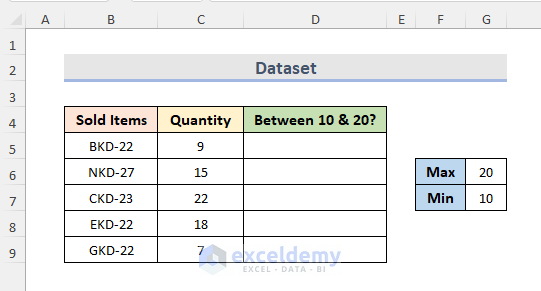
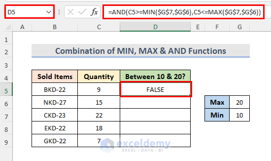
Assuming we have a dataset (B4:D9) of a company’s sold items with their quantity. Now, we will check whether the quantity of each sold item is between 10 and 20. We will see the result in column D. Here in the dataset, cells G6 and G7 contain the Maximum (20) & Minimum (10) values respectively.
1. Check If Value Is Between 10 and 20 Using IF Function
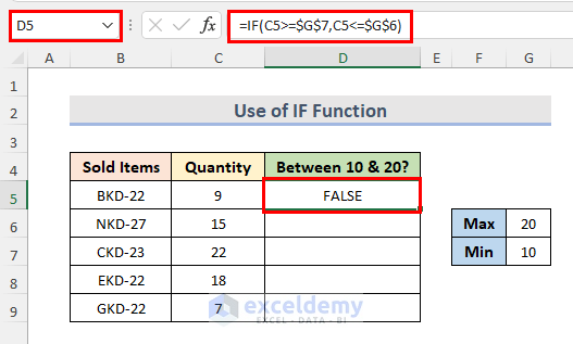
We know that the IF function helps us to run a logical test as well as returns TRUE for one value and FALSE for another one. We will use this function to get the value between 10 & 20.
Steps:
- First, select cell D5.
- Now write down the formula:
=IF(C5>=$G$7,C5<=$G$6)- Then press Enter to see the result.
- Here, we will see a small green box at the bottom corner of cell D5. If we hover a mouse on it, we can see that it turns into Black Plus (+) sign.
- Next, left-click the mouse and drag down the plus sign.
- After that, release the mouse.
- Finally, we can see the result in column D.

2. Insert AND Function to Find Out Value Between 10 and 20 in Excel
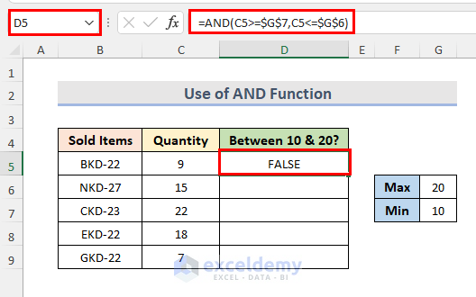
The AND function is one of the most frequently used functions in Excel. In this dataset, it will return TRUE if the values are between 10 & 20; otherwise FALSE.
Steps:
- In the beginning, select cell D5.
- Next, type the formula:
=AND(C5>=$G$7,C5<=$G$6)- Now press Enter.
- In the end, use the Fill Handle tool to see the result.

3. Detect Values Between 10 and 20 in Excel Using IF and AND Functions
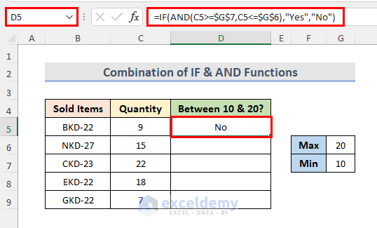
In this method, we will use the IF function and the AND function to determine if the value is between 10 & 20. Let’s see how to do this.
Steps:
- First, select cell D5.
- After that, write down the below formula:
=IF(AND(C5>=$G$7,C5<=$G$6),"Yes","No")- Then press Enter.
- Further, use the Fill Handle to autofill the below cells.

4. Combination of MIN, MAX & AND Functions to Look If the Value Is Between 10 and 20
The MAX function returns the maximum value whereas the MIN function returns the minimum value of the given argument. Here, we can combine these two functions with the AND function to see if the value is between 10 & 20 or not.
Steps:
- Select cell D5.
- Now, enter the below formula:
=AND(C5>=MIN($G$7,$G$6),C5<=MAX($G$7,$G$6))- After that, press Enter.
- Next, apply the Fill Handle tool to the below cells.

🔎 How Does the Formula Work?
- C5>=MIN($G$7,$G$6): This will check whether the cell C5 is greater than or equal to the minimum value in the G6:G7 range and return FALSE.
- C5<=MAX($G$7,$G$6): This will check whether the cell C5 is less than or equal to the maximum value in the G6:G7 range and return TRUE.
- AND(C5>=MIN($G$7,$G$6),C5<=MAX($G$7,$G$6)): This part will evaluate the condition of the cell C5 and return FALSE.
5. Apply Conditional Formatting in Excel to Highlight Value Between 10 and 20
Excel Conditional Formatting helps us apply specific formatting to a range. Let’s see how to apply it to our dataset.
5.1 Use Formula
We will use the AND function with Conditional Formatting to highlight values between 10 & 20. Follow the below steps.
Steps:
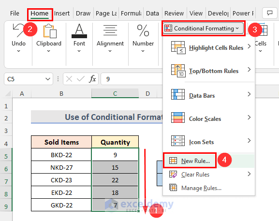
- First, select the range C5:C9 of quantity.
- Next, go to the Home tab.
- Select the Conditional Formatting drop-down.
- Now select the New Rule.
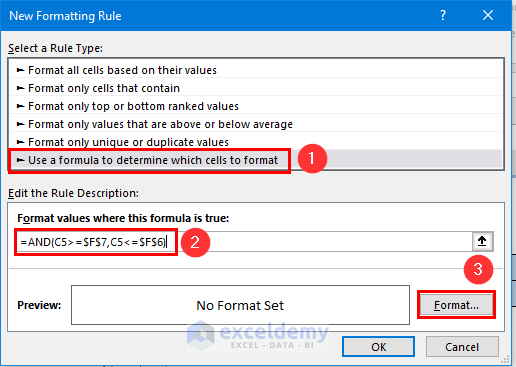
- A New Formatting Rule window pops up. Go to Use a formula to determine which cells to format option.
- In the formula box, type the formula:
=AND(C5>=$F$7,C5<=$F$6)- Select the Format option.
- Further, from the Format Cells window, go to the Fill tab.
- After that, select a background color.
- Consequently, we can see the color preview from the Sample option.
- Click on OK.

- Again, click on OK.

- Finally, we can see the result.

5.2 Apply Highlight Cells Rules Option
Excel has some built-in features to make the calculation easier. Conditional Formatting is one of them. We are going to follow the steps below.
Steps:
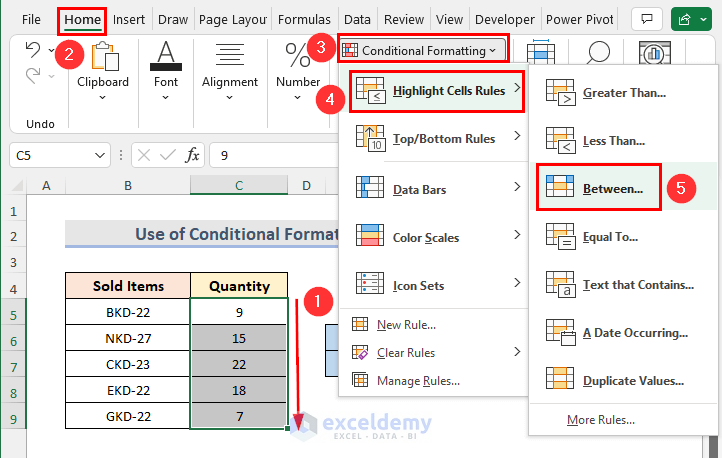
- Select the range C5:C9.
- Now go to the Home tab > Conditional Formatting drop-down.
- Select the Highlight Cells Rules option.
- Then click on the Between.
- We can see a Between window pops up.
- Further, input the numbers (10 & 20) in Format cells that are BETWEEN section.
- Also, select any color. Here we have selected Yellow Fill with Dark Yellow Text option.
- At last, click on OK.

- Consequently, we can see that all the cells containing values between 10 & 20 are highlighted. See the screenshot below for a better understanding.

How to Count Value Between 10 and 20 in Excel
Suppose, we want to count the cells that contain the value between 10 & 20 in Excel. We use different types of Excel functions here to perform the job. Here, we used the same dataset as above.
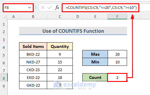
1. Insert COUNTIFS Function
The COUNTIFS function counts the cells in an array or range that matches the multiple criteria. It is tagged under Excel Statistical functions. Let’s see how to apply this to our dataset.
Steps:
- In the beginning, select cell F8.
- Further, enter the below formula:
=COUNTIFS(C5:C9,"<=20",C5:C9,">=10")- Next, hit Enter to see the result. In our case, it’s 2.
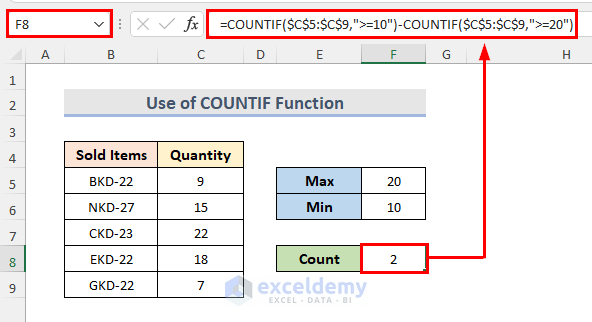
2. Use COUNTIF Function
The COUNTIF function counts the cells in an array or range that matches a single criterion. That means the exact use of the COUNTIF function accepts only one argument. Suppose, we have the same dataset as before. Now we are going to apply the COUNTIF function.
Steps:
- First, select cell F8.
- After that, write the below formula:
=COUNTIF($C$5:$C$9,">=10")-COUNTIF($C$5:$C$9,">=20")- Then, hit Enter. We can see that the result is 2.
Download Practice Workbook
Download the practice workbook from here.
Conclusion
Using these methods, we can quickly check if the value is between 10 and 20 in Excel. There is a practice workbook that we added. Go ahead and give it a try. Feel free to ask anything or suggest any new methods.
<< Go Back to Excel IF Function | Excel Functions | Learn Excel
Get FREE Advanced Excel Exercises with Solutions!
