If you are looking for ways to apply Conditional Formatting with the AND function in Excel, then this article will serve this purpose. Sometimes you may need to highlight cells only when they fulfill both conditions at a time. So, let’s get into the main article.
How to Use Conditional Formatting with AND Function in Excel: 4 Ways
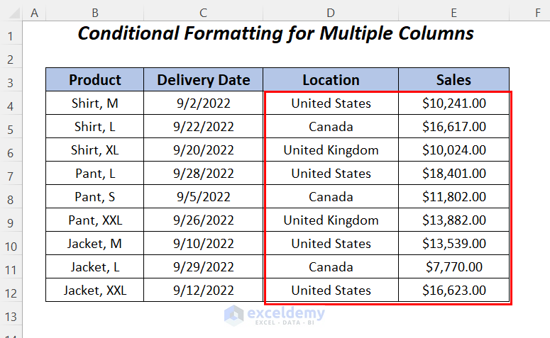
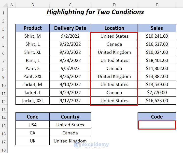
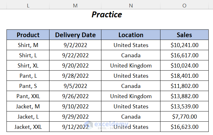
Here, we have the following dataset containing a list of products, their corresponding delivery dates, locations to be delivered, and their estimated sales values. Using this dataset, we will try to apply various conditions to highlight using conditional formatting.
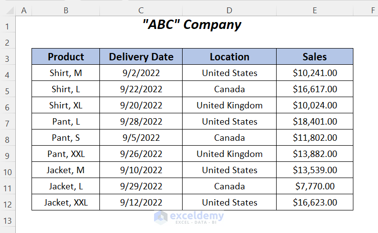
We have used Microsoft Excel 365 version for creating this article. However, you can use any other version at your convenience.
Method-1: Using AND Function to Apply Conditional Formatting in a Single Column
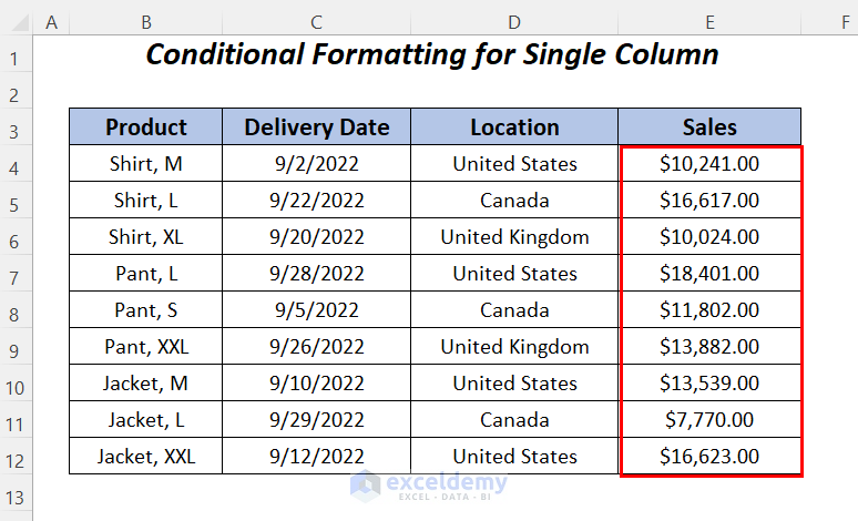
Here, we will highlight the rows having sales values greater than 10,000 USD and smaller than 15,000 USD by using the AND function to specify these two conditions in the Sales column.
- Select the range and then go to the Home tab >> Conditional Formatting dropdown >> New Rule

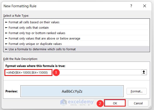
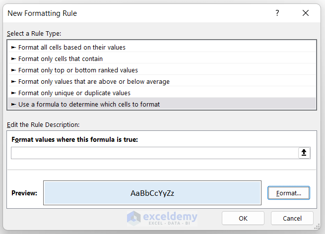
After that, the New Formatting Rule dialog box will open up.
- Choose the option Use a formula to determine which cells to format.
- Click on Format.

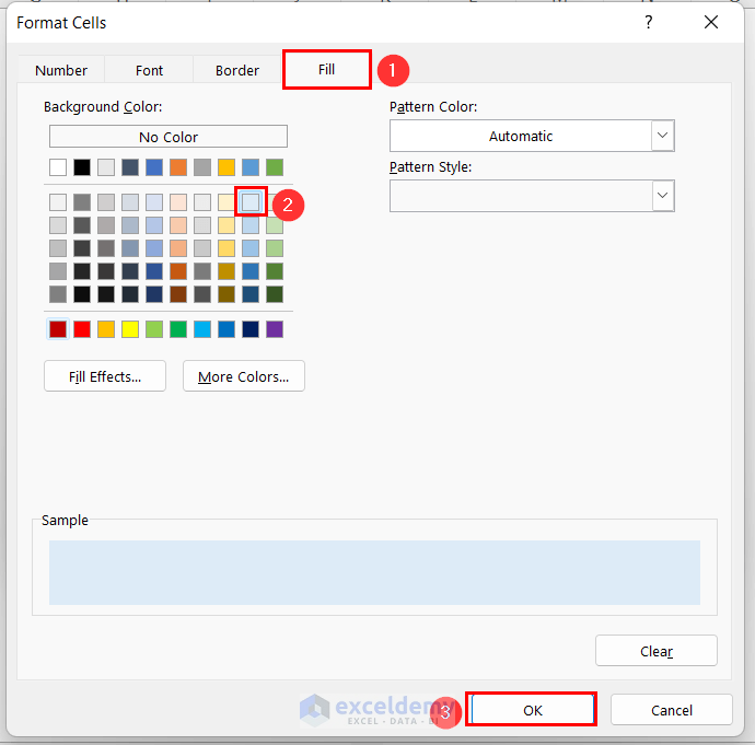
In this way, the Format Cells wizard will pop up.
- Go to the Fill tab >> choose Blue, Accent 5, Lighter 80% color >> press OK.
Then, you will be taken to the New Formatting Rule dialog box again.

Step-02:
- Type the following formula in the Format values where this formula is true
=AND($E4>10000,$E4<15000)When these two conditions are fulfilled, AND will return TRUE, and the corresponding rows will be highlighted.
- Press OK.
Finally, the rows that have sales values greater than 10,000 USD and smaller than 15,000 USD will be highlighted.

Read More: How to Return TRUE or FALSE Using Excel AND Function
Method-2: Using AND Function to Apply Conditional Formatting in Multiple Columns
Here, we will highlight the rows which have Canada as the Location, and sales values greater than 10,000 USD.
Steps:
- Follow Step-01 of Method-1.
Then, you will get the following preview of the New Formatting Rule dialog box.
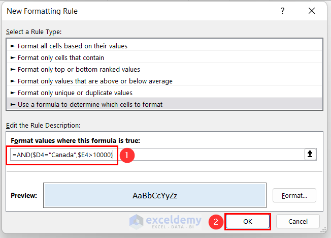
- Type the following formula in the Format values where this formula is true
=AND($D4="Canada",$E4>10000)When the country of the Location column is Canada and the Sales values of the Sales are greater than 10,000 USD. AND will return TRUE, and the corresponding rows will be highlighted.
- Press OK.
Finally, you will get the highlighted rows for Canada and sales values greater than 10,000 USD.

Read More: How to Use IF with AND Function in Excel
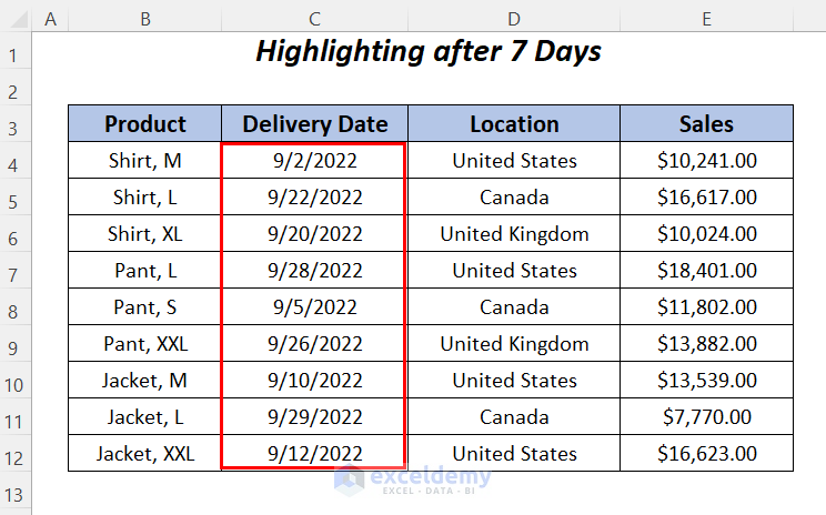
Method-3: Highlighting Dates within 7 Days
Here, we will highlight the dates which are situated within 7 days of today (9/22/2022 as mm/dd/yyyy format). By using the TODAY function we will extract today’s date and then apply the conditions to notify the upcoming delivery dates within 7 days.
Steps:
- Follow Step-01 of Method-1.
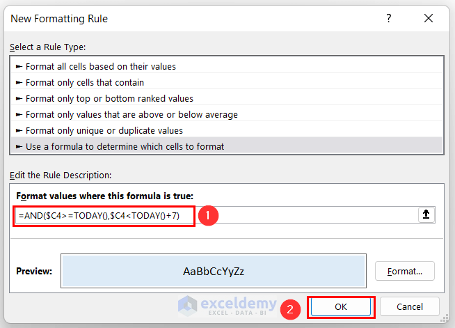
Then, you will get the following preview of the New Formatting Rule dialog box.

- Type the following formula in the Format values where this formula is true
=AND($C4>=TODAY(),$C4<TODAY()+7)When a date is greater than or equal to today’s date and less than the date after 7 days from today, AND will return TRUE, and the corresponding rows will be highlighted.
You can insert 15, 30, or whatever days you need.
- Press OK.
Afterward, you will get the following highlighted dataset showing the upcoming delivery dates within 7 days.

Read More: How to Use IFS and AND Functions Together in Excel
Method-4: Applying Conditional Formatting with AND Function for Two Conditions
Here, we will insert a code of a corresponding country’s name, and then depending on this code, we will highlight the full name of the countries in the Location column.
Step-01:
Firstly, we will create a dropdown list of codes in cell E15.
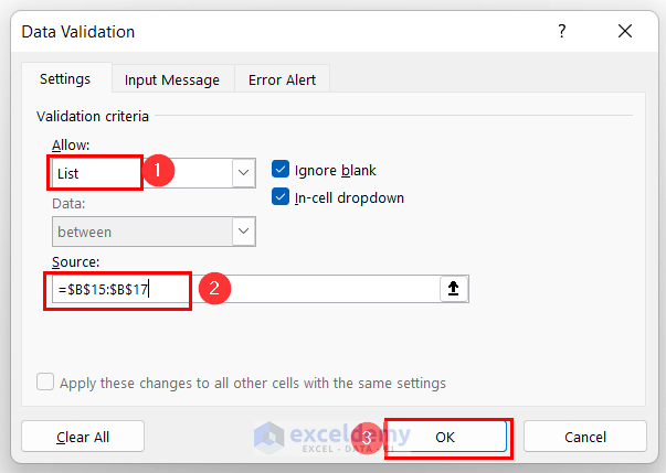
- Select cell E15, and then go to the Data tab >> Data Tools group >> Data Validation.

After that, you will have the Data Validation dialog box.
- Select List from different Allow
- In the Source box type the following formula or select the range of the codes.
=$B$15:$B$17- Press OK.
After that, the dropdown symbol will appear in cell E15.
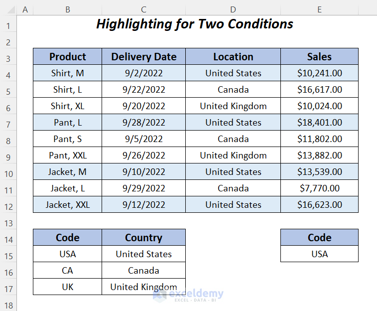
- Click on the dropdown symbol and select USA.

Then, the USA will appear in cell E15.

Step-02:
- Follow Step-01 of Method-1.
Then, you will get the following preview of the New Formatting Rule dialog box.

- Type the following formula in the Format values where this formula is true
=OR(AND($E$15=$B$15,$D4=$C$15),AND($E$15=$B$16,$D4=$C$16),AND($E$15=$B$17,$D4=$C$17))Three AND functions are used for each code and their country names. Finally, the OR function will highlight the rows when any of these conditions become TRUE.
- Press OK.

Finally, the rows with the country United States for the code USA will be highlighted.
If we change the code to CA, the rows corresponding to Canada will be highlighted.

Practice Section
For doing practice, we have added a Practice portion on each sheet on the right portion.
Download Workbook
Conclusion
In this article, we tried to show the ways to apply Conditional Formatting with the AND function in Excel. Hope you will find it useful. If you have any suggestions or questions, feel free to share them in the comment section.
Related Articles
- How to Use AND Function with Text in Excel
- Nested IF and AND Functions in Excel
- How to Use SUMIF and AND Function in Excel
<< Go Back to Excel AND Function | Excel Functions | Learn Excel
Get FREE Advanced Excel Exercises with Solutions!
