How to Use IFS and AND Functions Together in Excel (3 Examples)

Syntax of IFS and AND Functions

The syntax for the IFS function is given below.

=IFS(logical_test1, value_if_true1, [logical_test2, value_if_true2],...)

The IFS function can test several arguments at a time whether it is true or not. If the argument meets the criteria, the function returns the ‘value_if_true’ value. Otherwise, it returns the Value not Available Error (#N/A). To get rid of this problem, we state the logical_test that does not meet any arguments of the system as TRUE and then put the ‘value_if_true’ value for that logical_test.

Let’s have a simple example to illustrate this issue. Suppose you want Apple as an output in cell B5 if you type A in B4. For any other character, it will return nothing. So, the first logical_test will be if the cell value of B4 matches with A. We can express this logical_test as B4=“A”. The next thing will be the output (Apple) we want if the cell value of B4 matches the condition. We write this as “Apple” after the logical_test. The next logical_test will be if the value in B4 does not match with the letter A. Following the description above, we can express this as TRUE and put a space (“ ”) in the value_if_true argument.

The formula will look like this

=IFS(B4="A","Apple",TRUE,"")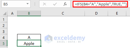

The syntax for the AND function is given below.

=AND(logical1, [logical2])

The function checks whether all the arguments are TRUE, and returns TRUE if all arguments are TRUE. Otherwise, it returns FALSE.

How to Use IFS and AND Functions Together in Excel: 3 Examples

Method 1 – Applying Excel IFS and AND Functions Together to Determine CGPA

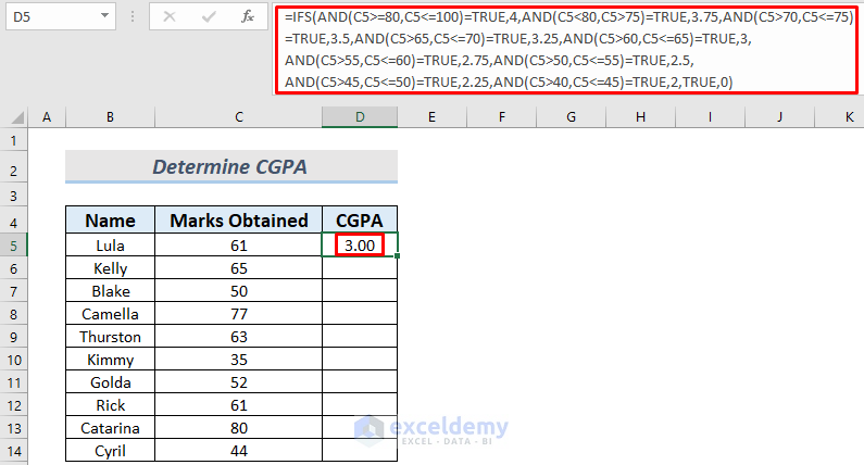
Suppose you are a teacher and you want to determine the Grade Point of the students based on their Obtained Marks.

Steps:

Make a column to store the Grade Points, copy the following formula in cell D5, then press Enter:

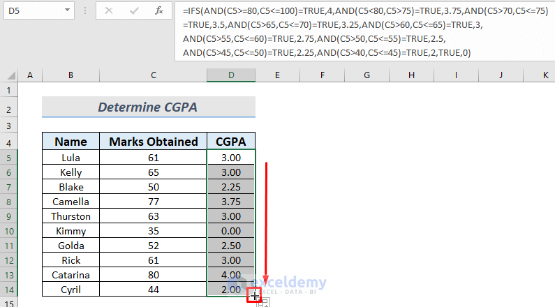
=IFS(AND(C5>=80,C5<=100)=TRUE,4,AND(C5<80,C5>75)=TRUE,3.75,AND(C5>70,C5<=75)=TRUE,3.5,AND(C5>65,C5<=70)=TRUE,3.25,AND(C5>60,C5<=65)=TRUE,3,AND(C5>55,C5<=60)=TRUE,2.75,AND(C5>50,C5<=55)=TRUE,2.5,AND(C5>45,C5<=50)=TRUE,2.25,AND(C5>40,C5<=45)=TRUE,2,TRUE,0)

Formula Breakdown

Although the formula looks horrible, let’s go through the arguments one by one. The formula returns the CGPA of the matched argument based on the Mark in C5.

AND(C5>=80,C5<=100)=TRUE, 4 —-> returns the Grade Point 4.00 if the mark is in the range [80, 100].
AND(C5<80,C5>75)=TRUE, 3.75 —-> returns the Grade Point 3.75 if the mark is in the range (75, 80).
AND(C5>70,C5<=75)=TRUE, 3.5 —-> returns the Grade Point 3.5 if the mark is in the range (70, 75].
AND(C5>65,C5<=70)=TRUE, 3.25 —-> returns the Grade Point 3.25 if the mark is in the range (65, 70].
AND(C5>60,C5<=65)=TRUE, 3 —-> returns the Grade Point 3.00 if the mark is in the range (60, 65].
AND(C5>55,C5<=60)=TRUE, 2.75 —-> returns the Grade Point 2.75 if the mark is in the range (55, 60].
AND(C5>50,C5<=55)=TRUE, 2.5 —-> returns the Grade Point 2.50 if the mark is in the range (50, 55].
AND(C5>45,C5<=50)=TRUE, 2.25 —-> returns the Grade Point 2.25 if the mark is in the range (45, 50].
AND(C5>40,C5<=45)=TRUE, 2 —-> returns the Grade Point 2.00 if the mark is in the range (40, 45].
TRUE, 0 —-> returns the Grade Point 0.00 if the mark is below 40.

Use the Fill Handle to AutoFill the lower cells.

Method 2 – Conditional Formatting Using Excel IFS and AND Functions Together

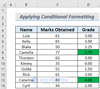
Say we want the CGPAs 4.00 and 3.75 to be filled with a green background color. We’ll use the dataset from the previous method.

Steps:

Select the range D5:D14.
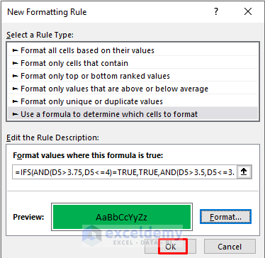
Go to Home, select Conditional Formatting, and choose New Rule.

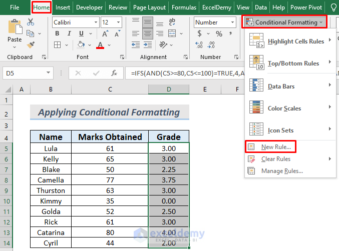
Select the Use a formula to determine which cells to format option in the New Formatting Rule dialog box.
Copy the following formula in the ‘Format values where this formula is true’ section:

=IFS(AND(D5>3.75,D5<=4)=TRUE,TRUE,AND(D5>3.5,D5<=3.75)=TRUE,TRUE)

The formula fills the cells with a color that satisfies the condition, which is the cells containing the CGPAs 4.00 and 3.75.

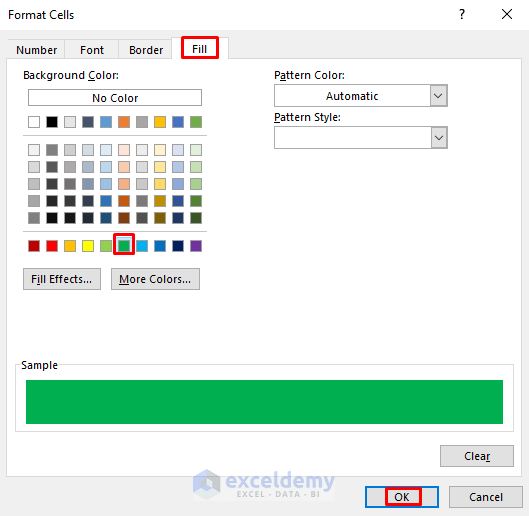
Click on Format.
Select the fill color from the Fill tab of the Format Cells. We chose Green.
You may format the Font too if you want.
Click OK.

The New Formatting Rule window will again pop up with a preview of how the formatted cells will look like.
Click OK.

You will see the Grade Points 4.00 and 3.75 filled with Green.

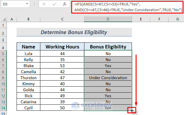
Method 3 – Using Excel IFS and AND Functions Together to Consider Bonus for Employee

Suppose you want to motivate your employees by giving them Bonuses to get their best effort. If someone works more than 47 hours a week, you will certainly give him a bonus. If someone works between 44 to 47 hours, you will decide later whether you give him a bonus or not. The other employees won’t receive any bonus.

Steps:

Make a column to store the Bonus Eligibility of your employees.
Copy the following formula in cell D5 and press Enter.

=IFS(AND(C5>47,C5<=53)=TRUE,"Yes",AND(C5<=47,C5>44)=TRUE,"Under Consideration",TRUE,"No")

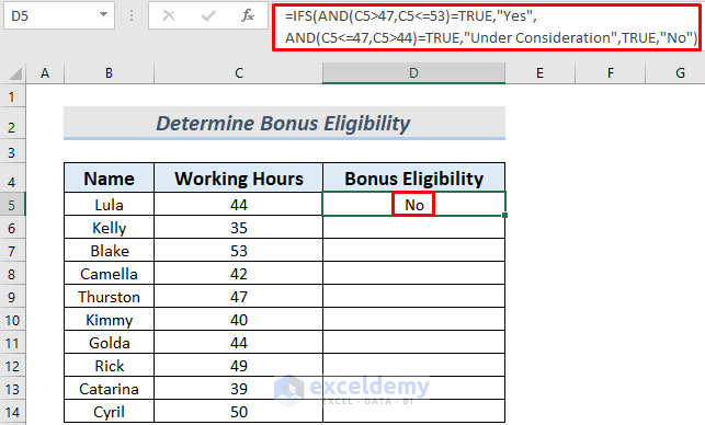
The formula will return the Bonus Eligibility for Lula. As they worked not more than 44 hours, they won’t get a bonus. And so, the Bonus Eligibility is “No”.