We often work with different conditions in Excel for accounting, business, or engineering purposes. And for that, we had to use some conditional functions like IF, COUNTIF, AND, SUMIF, and OR functions. In this tutorial, we’ll show three useful examples to learn how to use the AND function in Excel to return TRUE or FALSE for different kinds of conditions.
What Is AND Function?
The AND function of Microsoft Excel is used to return TRUE when all conditions turn TRUE. and It will return FALSE when any of the requirements are FALSE.
Introduction to AND Function in Excel
Purpose:
To return TRUE when all conditions turn TRUE and FALSE when any of the requirements are FALSE.
Syntax:
The syntax of the AND function is:
=AND(condition1, [condition2], … )
Arguments:
| Argument | Required/Optional | Explanation |
|---|---|---|
| condition1 | Required | The 1st condition for checking whether it’s TRUE or FALSE. |
| condition2 | Optional | Additional conditions for checking whether they turn TRUE or FALSE. Up to 30 conditions can be placed in total. |
Return Parameter:
Returns TRUE when all conditions turn TRUE.
And returns FALSE when any of the requirements turn FALSE.
Available in:
Available from Excel 2000.
How to Return TRUE or FALSE Using AND Function in Excel: 3 Examples
Now let’s see three practical examples to understand the application of the AND function.
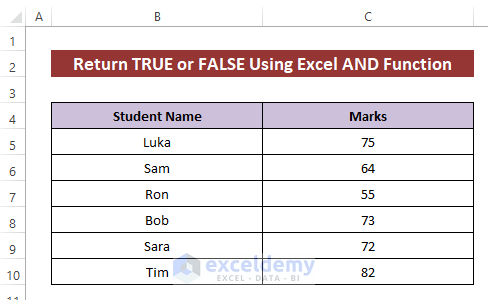
Example 1: Check a Value and Return TRUE or FALSE Using AND Function
Have a look at our dataset of the first method, it shows some students’ obtained numbers for an exam. We’ll apply the AND function to return TRUE if any number belongs between 70 to 80, otherwise will return FALSE.
Steps:
- In Cell D5, write the following formula in it-
=AND(C5>70,C5<80)- After hitting the ENTER button, we will get TRUE for Cell D5, as it meets the condition.
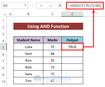
- Next, drag down the Fill Handle icon to copy the formula for the other cells.

Here’s our final output.

Example 2: Combine Excel AND and OR Functions to Return TRUE or FALSE
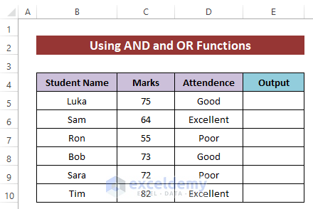
When we want to meet a condition independently then we use the OR function. And we can combine this function with the AND function for some cases. In this method, we’ll use them to find those students who have achieved a number more than 70 and have attendance in Good level or Excellent level. If these criteria meet then the formula will return TRUE otherwise FALSE. So, we modified the dataset as shown below.
Steps:
- Insert the following formula in Cell E5–
=AND(C5>70,OR(D5="Good",D5="Excellent"))- Then press the ENTER button to finish.

Formula Breakdown:
- OR(D5=”Good”,D5=”Excellent”)
The OR function will check the Cell D5 whether it contains ‘Good’ or ‘Excellent’. If contains one of them then it will return TRUE otherwise return FAlSE.
- AND(C5>70,OR(D5=”Good”,D5=”Excellent”))
Finally, the AND function will combine the output of the OR function and the logic C5>70, it will return TRUE if both logics return TRUE otherwise will return FALSE.
- After that, use the Fill Handle tool to get the other outputs.

3 students have met the condition. And it has provided TRUE for those students.

Read More: How to Use Conditional Formatting with AND Function in Excel
Example 3: Combine Excel IF and AND Functions to Return an Output
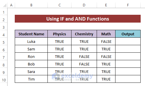
Imagine a scenario, we have three subjects’ results of the students, now we want to get the final result based on the subjectwise result. If any student failed in any subject then the formula will return ‘Failed’ otherwise will return ‘Passed’. To do that, we’ll use the IF function with the AND function.
We modified the dataset in that way and inserted the TRUE function to express passing and the FALSE function for expressing failed.
Steps:
- In Cell F5, write the following formula-
=IF(AND(C5=TRUE,D5=TRUE,E5=TRUE),"Passed","Failed")- Later, hit the ENTER button to get the result.

Formula Breakdown:
- AND(C5=TRUE,D5=TRUE,E5=TRUE)
The AND function will check each subject’s result for every student whether all are TRUE or not. If all gets TRUE then it will return TRUE otherwise will return FALSE.
- IF(AND(C5=TRUE,D5=TRUE,E5=TRUE),”Passed”,”Failed”)
Finally, the IF function will return ‘Passed’ for TRUE and ‘Failed’ for FALSE.
- To get the output for the other cells, use the Fill Handle tool.

Here’s our final result sheet, we got three failed students and three passed students.

Read More: How to Use IFS and AND Functions Together in Excel
Download Practice Workbook
You can download the free Excel template from here and practice independently.
Conclusion
That’s all for today. I hope all the methods described above will be good enough to use the AND function to get the desired output in Excel. Feel free to ask any question in the comment section and please give me feedback.
Related Articles
- How to Use AND Function with Text in Excel
- Nested IF and AND Functions in Excel
- How to Use SUMIF and AND Function in Excel
<< Go Back to Excel AND Function | Excel Functions | Learn Excel
Get FREE Advanced Excel Exercises with Solutions!
