Consider the following dataset with some order information. We’ll use SUMIF with AND to comb through the data.
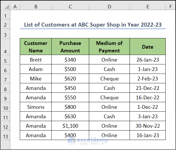
Example 1 – Application of SUMIF and AND Functions with Multiple Criteria
We will look for Online purchases, sum those values, then determine if they are above a threshold.
Steps:
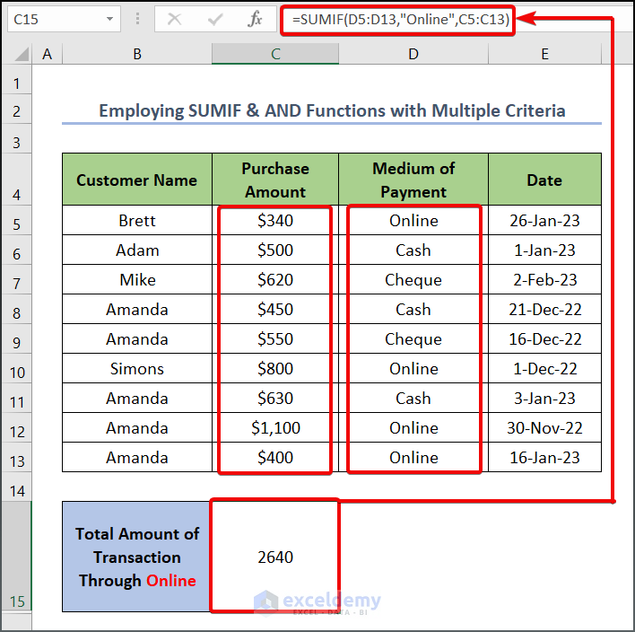
- In cell C15, use the following formula to calculate the accumulated value of Online transactions (column D).
=SUMIF(D5:D13,"Online",C5:C13)
Formula Breakdown:
- SUMIF(D5:D13,”Online”,C5:C13) → The SUMIF function adds the cells specified by a given criteria or condition. Here, D5:D13 is the range argument that refers to the Medium of Payment. The string “Online” refers to the criteria argument to apply within the given range. In this case, the formula will check if the value is equal to the criteria. C5:C13 is the optional sum_range argument, which indicates the corresponding value to sum if the value from range satisfies the criteria.
- Hit Enter.
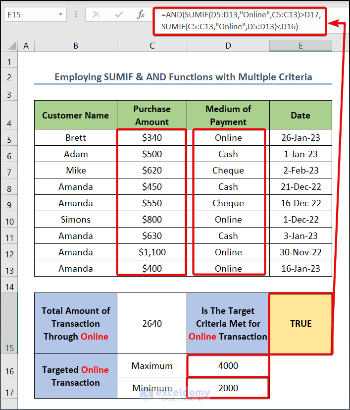
- Insert the sum benchmarks in cells D17 and D16 (lower and upper bound).
- In cell E15, use the following formula determine whether the total amount has met the requirement.
=AND(SUMIF(D5:D13,"Online",C5:C13)>D17,SUMIF(C5:C13,"Online",D5:D13)<D16)
Formula Breakdown:
- AND(SUMIF(D5:D13,”Online”,C5:C13)>D17,SUMIF(C5:C13,”Online”,D5:D13)<D16) → checks whether all the arguments are TRUE and returns TRUE if all the arguments are TRUE. SUMIF(D5:D13,”Online”,C5:C13)>D17 checks if the value in the D17 cell is less than the total amount of transaction through Online, and SUMIF(C5:C13,”Online”,D5:D13)<D16 checks whether the value in the D16 cell is greater than the total amount.
- Since both arguments are TRUE, the AND function returns the output TRUE.
- Press Enter.
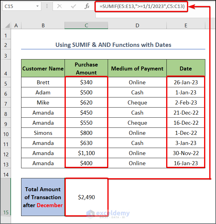
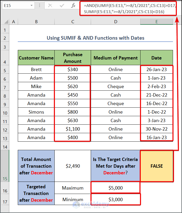
Example 2 – Application of SUMIF and AND Functions with Dates
Steps:
- Use the following formula in cell C15 to sum all the sales made on or after December 1, 2023.
=SUMIF(E5:E13,”>=1/1/2023″,C5:C13)
Formula Breakdown:
- SUMIF(E5:E13,”>=1/1/2023″,C5:C13)→ The string “>=1/1/2023” refers to the criteria argument to apply within the given range. It checks whether each cell in the range E5:E13 has a value higher than the date of 1/1/2023, then sums up the corresponding value from C5:C13.
- Press Enter.
- Insert the value benchmarks in D16 and D17 (upper and lower bound).
- Use the following formula in cell E15.
=AND(SUMIF(E5:E13,">=8/1/2021",C5:C13)>D17,SUMIF(E5:E13,">=8/1/2021",C5:C13)<D16)
Formula Breakdown:
- AND(SUMIF(E5:E13,”>=8/1/2021″,C5:C13)>D17,SUMIF(E5:E13,”>=8/1/2021″,C5:C13)<D16)
- The SUMIF functions calculate the sum of values after August 1, 2021.
- AND compares the result against the benchmarks and returns the output TRUE if the value is between D16 and D17 (done by comparing SUM>D16 AND SUM<D17).
- Hit Enter.
Read More: Nested IF and AND Functions in Excel
Things to Remember
- The AND function can take up to 255 arguments as its logical condition.
- If you provide an array condition into the SUMIFS function which simultaneously discovers a merged cell as the return destination, a #SPILL error will occur.
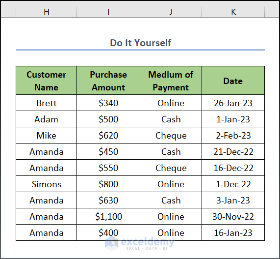
Practice Section
We have provided a Practice section on the right side of each sheet to test these methods.
Download the Practice Workbook
Related Articles
- Use IF with AND Function in Excel
- How to Use IFS and AND Functions Together in Excel
- Return TRUE or FALSE Using Excel AND Function
- How to Use Conditional Formatting with AND Function in Excel
- Use AND Function with Text in Excel
<< Go Back to Excel AND Function | Excel Functions | Learn Excel
Get FREE Advanced Excel Exercises with Solutions!
