How to Use Excel Formula Not to Exceed a Certain Value

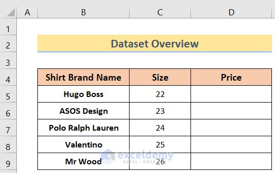
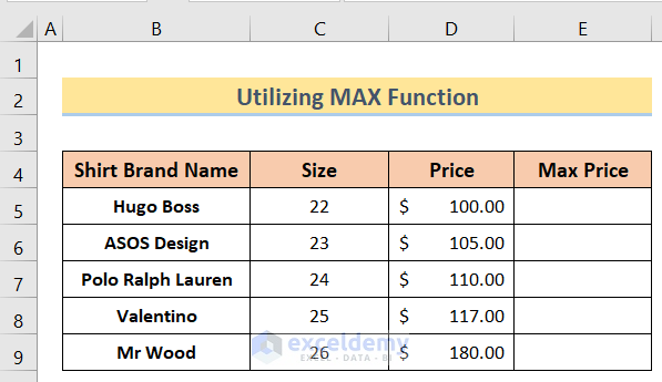
We’ll use the following sample dataset, which contains Shirt Brand Names in Column B, Sizes in Column C, and Prices in Column D.

Method 1 – Using a Data Validation Value Range

If we want to record the age of customers in a cell range, we can set the Data Validation to accept numerical values only, set upper and lower limits for a particular type of data, and return a message to the user about why the data was not accepted and how to resolve the issue.

Steps:

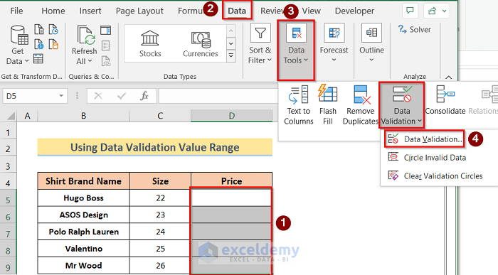
• Select the range Size.
• Click the Data Tab.
• Click Data Tools.
• Select Data Validation from the drop-down list.
• Select Data Validation from the Data Validation drop-down list.

The Data Validation window will pop up on the screen.

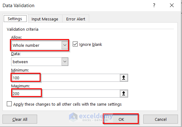
• Click the Settings tab.
• Select Whole Number under Validation Criteria Allow.
• Select between under Data.
• Enter 100 as Minimum.
• Enter 200 as Maximum.

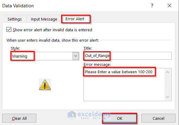
• Click the Error Alert tab.
• Select Warning from the Style drop-down menu.
• Put Out_of_Range as Title.
• Enter “Please Enter a value between 100–200” for Error message.
• Press OK.

If you enter a value outside the accepted range (100 to 200), the warning message will display.

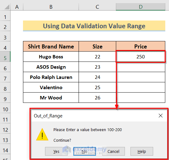
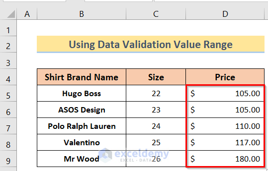
• Enter values into the other cells in column D manually. Only values within the range 100 to 200 will be accepted.

Method 2 – Using a Data Validation Custom Formula

Steps:

• As in the previous method, select the range Size and choose Data Validation.

The Data Validation window will pop up on the screen.

• In the Settings tab, select Custom under Allow.
• Enter the following formula under Formula:

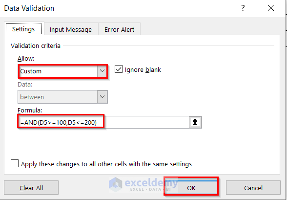
• Click OK,
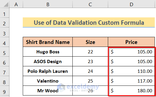
• Start inserting values manually in column D.

Only values within the range will be accepted.

Method 3 – Using the MAX Function

Steps:

• Arrange the dataset as per the below image.

• Enter the following formula in cell E5:

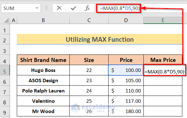
• Press Enter to return the result.
• Drag the Fill Handle down to apply the formula to the other cells in column E.

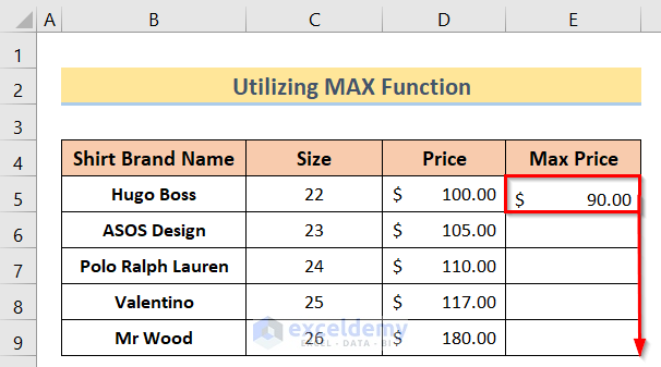
• The Maximum Prices will be set by our formula (the greater of 90 and 80% of the Price).

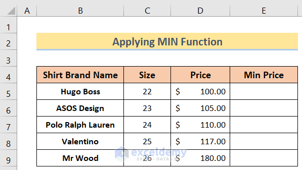
Method 4 – Using the MIN Function

Steps:

• Arrange the dataset like the below image.

• Insert the following formula in cell E5:

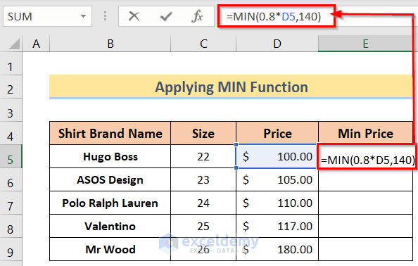
• Press Enter to return the result.
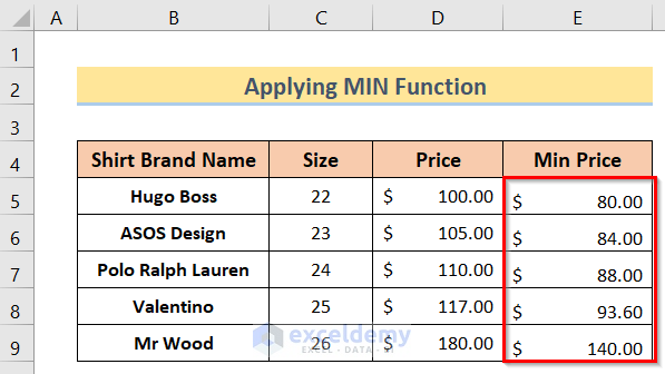
• Drag the Fill Handle down to apply the formula in the rest of the cells in the column.

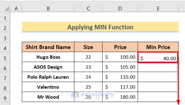
Minimum Prices are set (the lower of 140 and 80% of the Price).

Method 5 – Using the IF Function

Steps:

• Arrange the dataset like the below image.

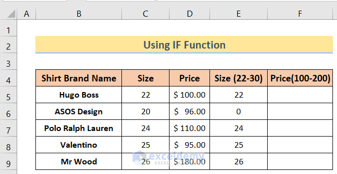
• Insert the following formula in cell F5:

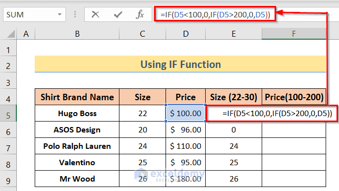
• Press Enter.
• Drag the Fill Handle down to apply the formula to the other cells in the column.

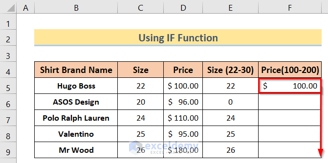
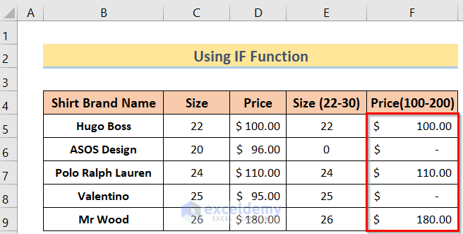
The results are as follows:

Method 6 – Using the RANDBETWEEN Function

Steps:

• Arrange the dataset like the below image.

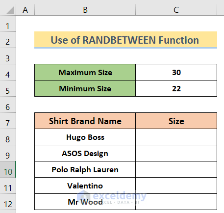
• Insert the following formula in cell C8:

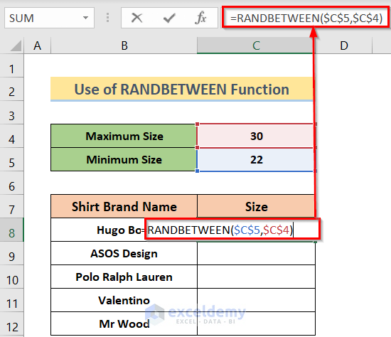
• Press Enter to return the result.
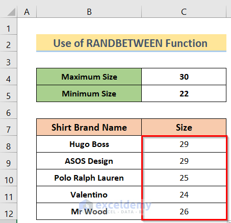
• Drag the Fill Handle down to apply the formula to the rest of the cells in the column.

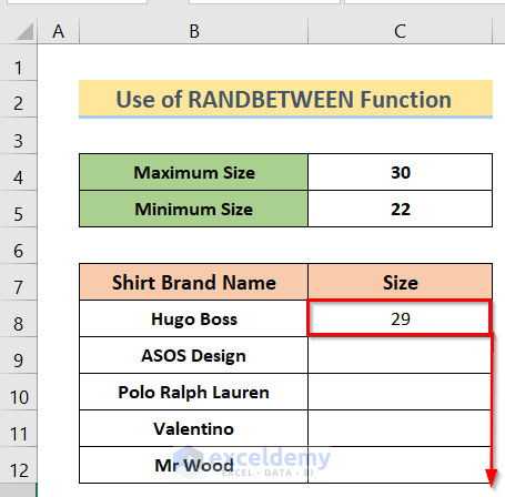
The results are as follows:

Download the Practice Workbook

Related Articles

• How to Make a Data Validation List from Table in Excel
• Excel Data Validation Drop-Down List
• Excel Data Validation Drop Down List with Filter
• How to Use Data Validation List from Another Sheet

<< Go Back to Data Validation in Excel | Learn Excel