I Tried Rebuilding a Power BI Report in Excel: Here’s Where It Failed (and Where It Didn’t)

 

Power BI is popular for interactive reports and dashboards. But as an Excel lover, I wonder, “How far can Excel go if I try to recreate a Power BI report?”. I attempted to recreate a typical Power BI sales report within Excel using Power Query, the Data Model (Power Pivot), DAX measures, PivotTables/Charts, Slicers/Timelines, and some layout polish.

In this article, I will show how I tried to rebuild a Power BI report in Excel and where it failed and where it didn’t.

The Report I Tried to Recreate

A standard sales overview with:

• KPI cards: Total Sales, Total Profit, Profit Margin, etc.
• Trend line: Sales by Month.
• Breakdown: Sales by Category, by Region, etc.
• Interactivity: Slicers for Year, Category, Region, and a date timeline.
• Drill to detail: A detailed view filtered by current selections.

This type of dashboard is commonly used; many teams build in Power BI. Let’s mirror it in Excel. The goal was to see if I could reproduce both the functionality and the user experience in Excel.

Step 1: Load & Clean with Power Query (Get & Transform)

• Go to the Data tab >> select Get Data >> select From Text/CSV or other sources.
• Browse and select the file and import file.
• Click Load or Transform Data to clean the dataset.

• In Power Query Editor, set types properly (Date, Whole Number, Currency).
• Clean your data with small fixes: trim text, standardize casing, etc.

• Click Close & Load To…to import the data.
• Then select the required options;
  • Table or Only Create Connection.
  • Add this data to the Data Model.
  • Click OK.

• Import all data following the same steps.

Where Excel Succeeded:

• Power Query functionality is identical to Power BI.
• Data transformation capabilities are robust.
• Multiple data source connections work well.

Where Excel Failed:

• No incremental refresh options.
• Limited to 1 million rows per worksheet.
• Slower performance with large datasets.
• Manual refresh required (no gateway scheduling).

Step 2: Build Relationship in the Data Model (Power Pivot)

• Go to the Data tab >> select Manage Data Model.
• Or go to the Power Pivot tab >> select Manage.

• Add relationships:
  • Sales[ProductID] → Products[ProductID]
  • Sales[CustomerID] → Customers[CustomerID]
  • Customers[RegionID] → Regions[RegionID]

• Hide keys and technical columns from client tools to maintain clean field lists.

Power BI: It automatically detects and creates relationships. For further adjustment, you can drag-and-drop to create relationships.

Excel: Power Pivot provides similar relationship modeling. It may seem like a more complex interface for managing relationships.

Step 3:  Create DAX Measures

In the Data Model, you can create DAX measures. Either you can create DAX measures in the Power Pivot formula bar, or you can use the calculations option.

• Go to the Power Pivot >> from Calculations >> select Measures >> select New Measure.
• Insert the measure name and the formula.
• Click OK.

Total Sales = SUM(Sales[SalesAmount])

Total Cost = SUM(Sales[Cost])

Profit = [Total Sales] - [Total Cost]

Profit Margin % = DIVIDE([Profit], [Total Sales])

Average Order Value = DIVIDE([Total Sales], DISTINCTCOUNT(Sales[OrderID]))

• Preview the formula and result in the Power Pivot window.

Power BI: The DAX measures work the same. Time intelligence functions light up as soon as you have a proper Calendar table related to Date.

Step 4: Build the Report Layer with PivotTables/Charts

• Insert a PivotTable connected to the Data Model.
  • Go to the Insert tab >> select PivotTable >> select Data Model.
  • Select location: Existing or New Worksheet.

• PivotTable is created in a new sheet.

Note: Remember to create different visuals, you must create separate PivotTables. One PivotTable doesn’t accommodate different visuals, which is time-consuming.

Create Visuals:

KPI Cards: 

• From the PivotTable Fields;
  • Drag the measures in Values.
  • Format as large font; hide grand totals/subtotals.

Create Interactive Charts:

• Create another PivotTable from the Data Model.
• Sales by Month:
  • Drag Date on Rows.
  • Drag SalesAmount in Values.
• Select the PivotTable.
• Go to the PivoTAnalyze tab >> select PivotChart >> select Line charts.
• Click OK.

• This chart gives drill-through experience using the Date hierarchy.

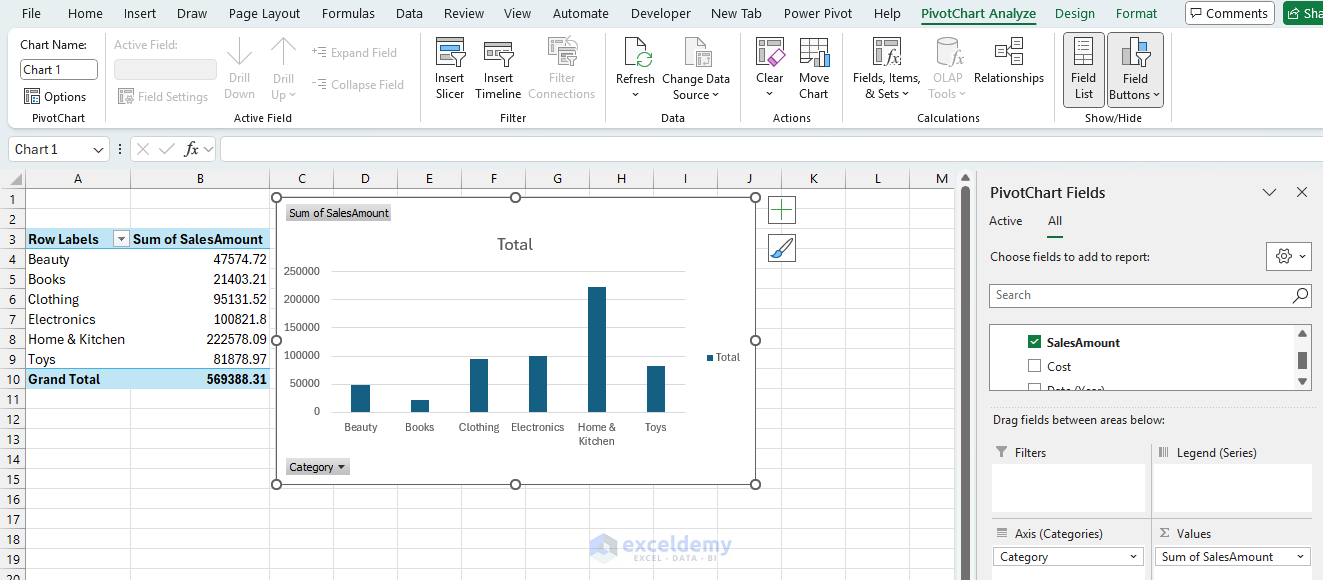
• Sales by Category/Region/Channel: Clustered column PivotCharts.
  • Drag Category on Rows.
  • Drag SalesAmount on Values.

• Sales by State/Province: Pie PivotCharts.
  • Drag State/Province on Rows.
  • Drag SalesAmount on Values.

• Map: You will need to create a Map chart from the static data.
  • Group Country and its SalesAmount, then use Excel’s Filled Map chart.

Power BI: Power BI offers next-level visualizations with interactivity. It offers the same core visuals, global slicers with a clean layout. It has built-in KPIs with traffic lights/icons tied to thresholds (without complex conditional formatting)

Where Excel Succeeded:

• More granular chart formatting control.
• Better text and annotation capabilities.
• Custom chart types through combination charts.
• Native sparklines functionality.

Where Excel Failed:

• No native map visualizations.
• Limited interactive visual types.
• No automatic chart legends with filters.
• Manual sizing and positioning required.
• No responsive design capabilities.

Step 5: Create Interactivity

• Add Slicers (Year, Category, Region) and a Timeline (Date).
  • Go to the PivotTable Analyze tab >> select Insert Slicer/Timeline.

• • Sync slicers across all PivotTables.
  • Go to the Slicer tab >> select Report Connections.
  • Or right-click Slicer >> select Report Connections.
  • Select all PivotTables and click OK.

Power BI: Click any visual to filter all others automatically. Also, it offers independent slicers along with formatting options.

Excel: Slicers work well for basic filtering. Multiple slicers can control multiple PivotTables, along with connections; they can create connectivity with other PivotTables. But there is no cross-visual filtering (clicking a chart doesn’t filter others). Limited drill-through capabilities and no bookmarking or view states.

Step 6: Arrange All Visuals to Create a Report

In Power BI, you can create all visuals in the report page; later, you just rearrange them, maintaining a strategic flow. In Excel, as we created multiple PivotTables, Slicers, charts, you will need to copy and organize these things into one or multiple sheets.

• Select the visual.
• Right-click >> select Copy.
• Select a place in the report sheet >> select Paste.
• Format all visuals to mirror the Power BI look.
• Excel offers plenty of formatting options.

• Try Interactivity by selecting Slicer.

Remember that all these PivotTables will slow down the performance. Loading time will increase significantly.

What Worked Surprisingly Well in Excel

• Data Import: The Power Query is similar to Power BI.
• Modeling & DAX: Star schema, time intelligence, and DAX measures are like Power BI.
• Core Visuals: Lines, bars, tables, KPI-style cards, and even a simple map are solid.
• Detail Exploration: Double-clicking a Pivot cell to “Show Details” (drill-through to rows) is handy, and a curated Detail sheet keeps it tidy.
• Performance (reasonable sizes): The Data Model is fast for typical departmental datasets.

Where Excel Fell Short (and Why It Matters)

• Cross-Highlighting Between Charts:
  • Power BI lets you click a bar in one visual to cross-filter and cross-highlight the others.
  • Excel’s slicers filter based on connections, but charts don’t highlight each other dynamically.
• Page-level Drill-through & Tooltips: 
  • Power BI’s Drill-through pages and Report Page Tooltips bring guided analysis.
  • Excel has none of that, but you can use hyperlinks to a detail sheet and clearly labeled slicers, yet it is still manual.
• Dynamic Field Parameters (dimension/measure switchers): 
  • Power BI’s field parameters are a joy.
  • In Excel, you can mimic with disconnected tables + SELECTEDVALUE + SWITCH, but it’s bulky and harder for end users to maintain.
• DirectQuery, Composite Models, Incremental Refresh:
  • Power BI can query big backends without importing everything, blend sources, and refresh incrementally.
  • Excel’s Data Model is import-only, and refresh happens all-or-nothing.
• Mobile-friendly, Bookmarks, Narratives: 
  • Power BI’s Bookmarked stories, selection pane tricks, and mobile layouts don’t translate.
  •  Excel requires VBA/hyperlinks for anything beyond simple navigation.

Quick Decision Guide

Choose Excel:

• Excel is better for analysis where a small team reports on OneDrive/SharePoint, but it doesn’t replace apps or mobile views.
• You need flexible and advanced calculations alongside the visuals (what-if cells, LAMBDA/LET, etc.).

Choose Power BI:

• If you need to share widely, refresh on a schedule, and control access per audience, Power BI Service is the clear win.
• It offers cross-highlighting, drill-through, tooltips, bookmarks, and mobile layouts. It can govern app distribution and usage of metrics.

Conclusion

Excel is a wonderful tool, and it meets the needs of basic to advanced-level users. It can mirror or rebuild a big slice of a typical Power BI report, especially the ETL, star schema, DAX, and core visuals. Where it fails is interactive storytelling, governed sharing, and enterprise-scale models/refresh. If your user, stakeholders live in Excel and the scope is contained, Excel is a perfectly credible reporting surface. But if you need click-through narratives, secure distribution, or live connections at scale, go for Power BI.