How to Use Formula for Car Loan Amortization in Excel (with Quick Steps)

We can easily calculate the car loan amortization by using the Microsoft Excel financial formulas. This is an easy task. While purchasing a car, sometimes we need to pay the payment of the car by some installment. We can easily pay the car loan amortization by applying Excel formula. This will save you a lot of time and energy. Today, in this article, we’ll learn four quick and suitable steps to calculate the car loan amortization in Excel effectively with appropriate illustrations.

Download Practice Workbook

Download this practice workbook to exercise while you are reading this article.

Introduction to the Loan Amortization

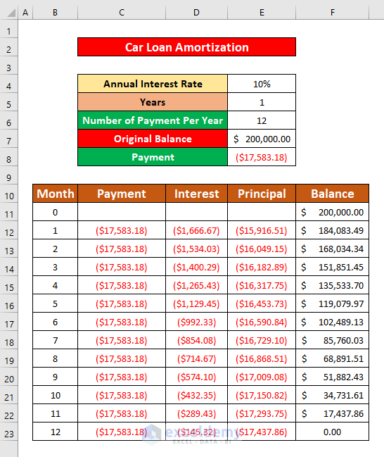
An amortizing loan is a loan where the principal is paid down throughout the life of the loan according to an amortization plan, often by equal payments, in banking and finance. An amortizing bond, on the other hand, is one that repays a portion of the principal as well as the coupon payments. Let’s say, the total value of the car is $200000.00, the annual interest rate is 10%, and you will pay the loan within 1 year.

4 Effective Steps to Use Formula for Car Loan Amortization in Excel

Let’s assume we have an Excel large worksheet that contains the information about the car loan amortization. From our dataset, we will calculate the car loan amortization by using the PMT, IPMT, and PPMT financial formulas in Excel. PMT stands for Payment, IPMT is used to get the interest of payment, and PPMT is used to get the principal payment. We will apply these financial functions to calculate the car loan amortization. Here’s an overview of the car loan amortization in the Excel dataset for today’s task.

We will do those four easy and quick steps, which are also time-saving. Let’s follow the instructions below to learn!

Step 1: Use the PMT Function to Calculate Principal of Car Loan Amortization in Excel

First of all, we will calculate the payment by using the PMT financial function. One can pay one’s payment every week, month, or year by using this function. The syntax of the function is,

=PMT(rate, nper, pv, [fv],[type])

Where rate is the interest rate of the loan, nper is the total number of payments per loan, pv is the present value i.e. the total value of all the loan payments at present, [fv] is future value i.e. the cash balance one wants to have after the last payment is done, and [type] specifies when the payment is due.

Let’s follow the instructions below to calculate payment by using the PMT function.

• First, select cell C11 and write down the PMT function in that cell. The PMT function is,

• Where E$4 is the Annual Interest Rate, E$6 is the number of payments per year, E$5 is the number of years, E$7 is the original price of the car. We use the dollar ($) sign for the absolute reference of a cell.

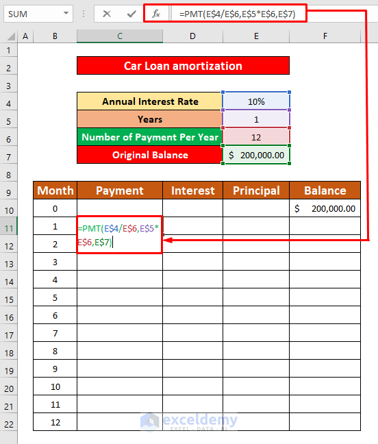
• Hence, simply press ENTER on your keyboard, and you will get the payment ($17,583.18) as the output of the PMT function.

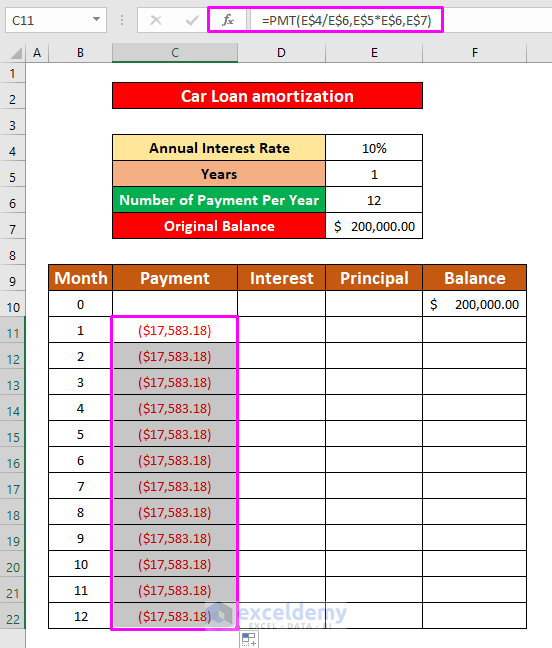
• Now, autoFill the PMT function to the rest of the cells in column C.

• After completing the above process, you will be able to calculate the payment of the loan per month which has been given in the below screenshot.

Read More: How to Use Formula for Mortgage Principal and Interest in Excel

Step 2: Apply the IPMT Function to Calculate Interest of Car Loan Amortization in Excel

After calculating the payment, now, we will calculate the interest of payment by applying the IPMT function. The syntax of the function is,

=IPMT(rate, per, nper, pv, [fv],[type])

Where rate is the interest rate per period, per is a specific period; must be between 1 and nper, nper is the total number of payment periods in a year, pv is the current value of a loan or investment, [fv]is the nper payments future worth, [type] is the payments behavior.

Let’s follow the instructions below to calculate the interest of payment by using the IPMT function.

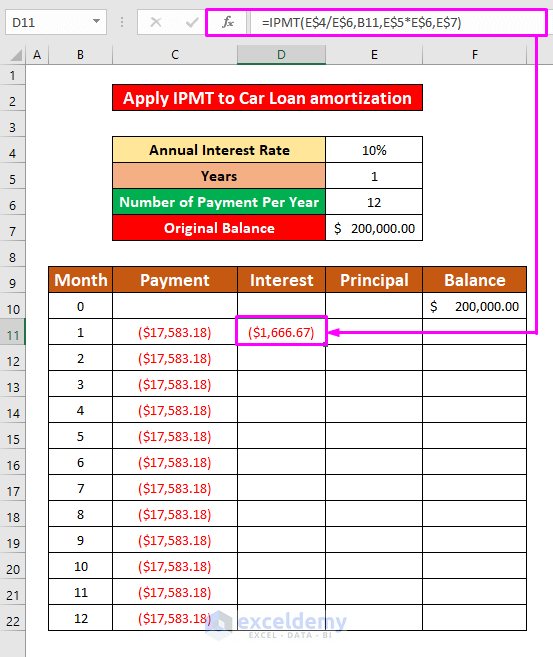
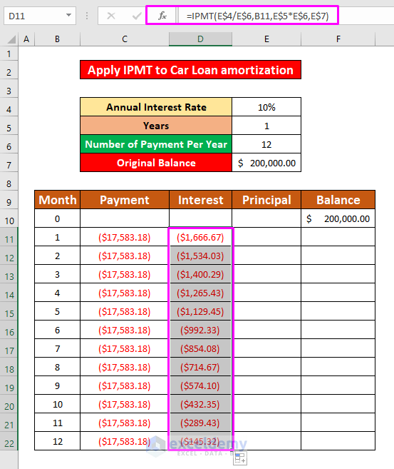
• First of all, select cell D11 and type the IPMT function in the Formula Bar. The IPMT function in the Formula Bar is,

• Where E$4 is the Annual Interest Rate, E$6 is the number of payments per year, B11 is the number of month, E$5 is the number of years, E$7 is the original price of the car. We use the dollar ($) sign for the absolute reference of a cell.

• Further, simply press ENTER on your keyboard, and you will get the interest of payment ($1666.67) as the output of the IPMT function.

• Hence, autoFill the IPMT function to the rest of the cells in column D.

• After completing the above process, you will be able to calculate the interest of payment of the car loan amortization per month which has been given in the below screenshot.

Read More: Interest Only Mortgage Calculator with Excel Formula (A Detailed Analysis)

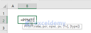
Step 3: Insert the PPMT Function to Calculate Interest of Car Loan Amortization in Excel

In this step, we will calculate the principal of payment by using the PPMT function. This is the easiest financial function. The syntax of the function is,

=IPMT(rate, per, nper, pv, [fv],[type])

Where rate is the interest rate per period, per is a specific period; must be between 1 and nper, nper is the total number of payment periods in a year, pv is the current value of a loan or investment, [fv]is the nper payments future worth, [type] is the payments behavior.

Let’s follow the instructions below to calculate the principal of payment by using the PPMT function.

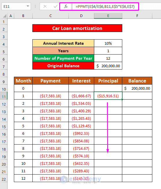
• First of all, select cell E11 and type the PPMT function in the Formula Bar. The PPMT function in the Formula Bar is,

• Where E$4 is the Annual Interest Rate, E$6 is the number of payments per year.
• B11 is the number of month.
• E$5 is the number of years, E$7 is the original price of the car.
• We use the dollar ($) sign for the absolute reference of a cell.

• After that, press ENTER on your keyboard, and you will get the interest of payment ($15916.51) as the output of the PPMT function.

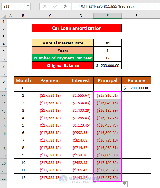
• Further, autoFill the PPMT function to the rest of the cells in column E.

• While performing the above process, you will be able to calculate the principal payment of the car loan amortization per month which has been given in the below screenshot.

Read More: Loan Amortization Schedule with Variable Interest Rate in Excel

Step 4: Use Formula for Car Loan Amortization in Excel

This is the final step to calculate the car loan amortization in Excel. After calculating the payment per month, interest of payment per month, and the principal payment per month, now, we will calculate the balance of the loan by using those values. Let’s follow the instructions below to calculate the balance by using the mathematical function.

• First of all, select cell F11 to apply the mathematical summation formula.

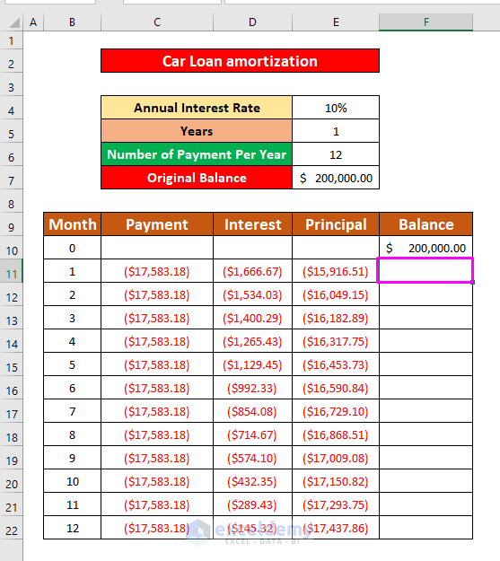
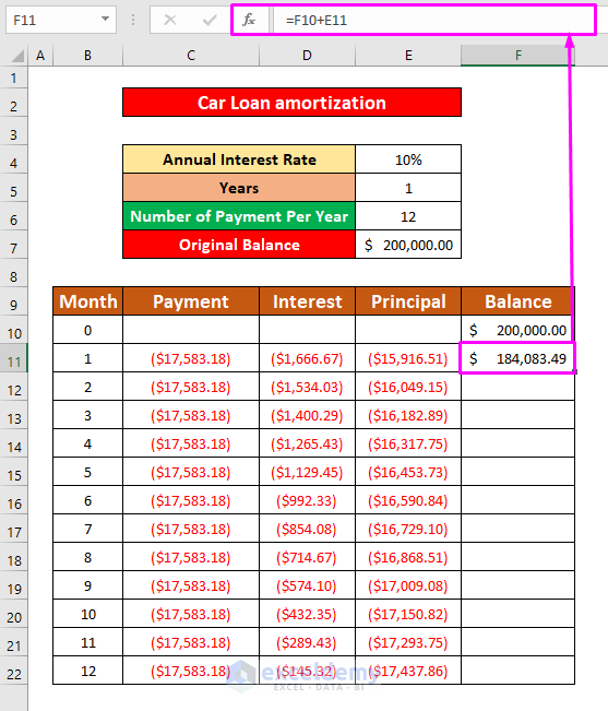
• After selecting cell F11, write down the following formula in the Formula Bar. The formula is,

• Where F10 is the initial price of the car, and E11 is the total payment after the first month.

• After that, press ENTER on your keyboard, and you will get the balance after the first month. The balance becomes $184,083.49 after the first month.

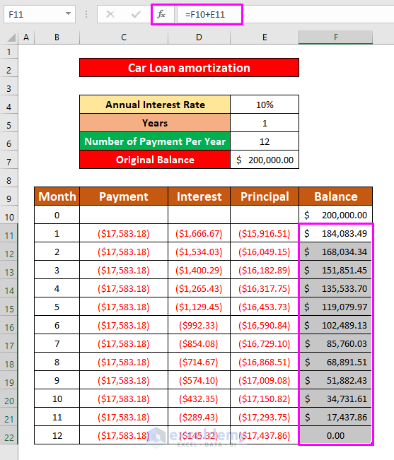
• While performing the above process, you will be able to calculate the car loan amortization per month. After the 12th month, you will be able to pay the total loan which has been given in the below screenshot.

Read More: Mortgage Calculations with Excel Formula (5 Examples)

Things to Remember

👉 #DIV/0 error occurs when the denominator is 0 or the reference of the cell is not valid.

👉 The #NUM! error occurs when the per argument is less than 0 or is greater than the nper argument value.

Conclusion

I hope all of the suitable steps mentioned above to use a formula for car loan amortization will now provoke you to apply them in your Excel spreadsheets with more productivity. You are most welcome to feel free to comment if you have any questions or queries.

Related Articles

• Creation of a Mortgage Calculator with Taxes and Insurance in Excel
• Mortgage Repayment Calculator with Offset Account and Extra Payments in Excel
• How to Use Formula for 30 Year Fixed Mortgage in Excel (3 Methods)
• Excel Interest Only Amortization Schedule with Balloon Payment Calculator
• Amortization Schedule with Balloon Payment and Extra Payments in Excel