How to Create Graphs in Excel
This is a sample dataset:
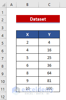
Steps
- Select B4:C11.
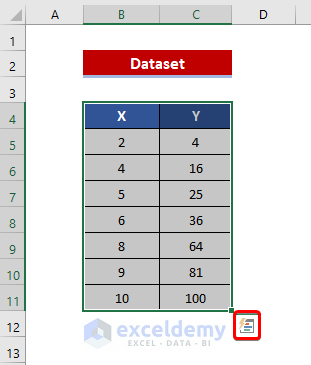
- The Quick Analysis option will be displayed at the right bottom corner.
- Click it.
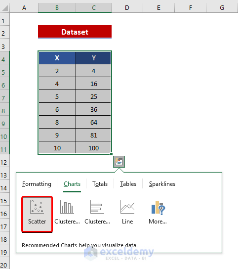
- Select the Charts tab and click Scatter.
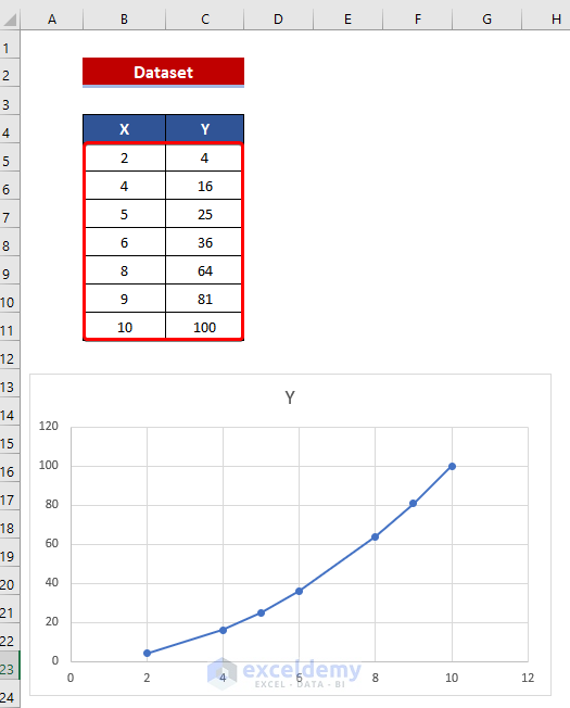
The chart based on the dataset is created.
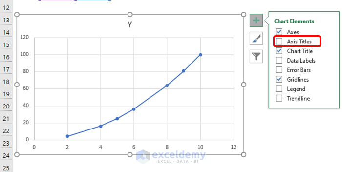
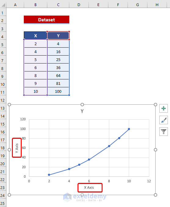
- Click the Axis Titles to see the X and Y axis. X is the horizontal axis and Y the vertical axis.
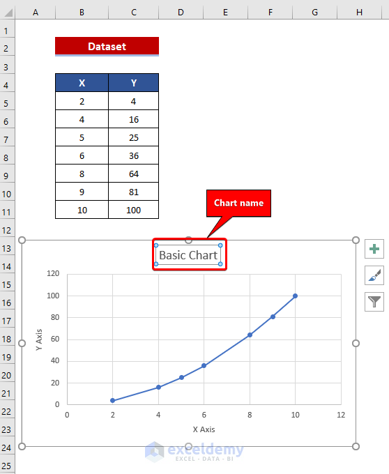
- To change the chart title, click it.
Read More: How to Add Secondary Axis in Excel
Combine Graphs with Different X Axis in Excel
This is the dataset:
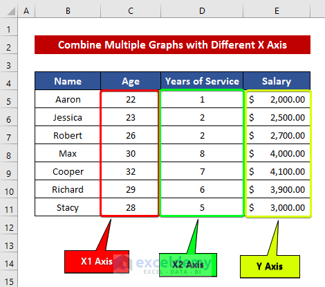
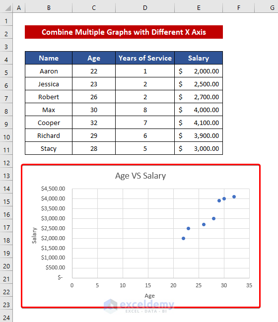
The dataset contains age, years of service, and salaries. There are two X horizontal axis. One is Age and the other Years of Service. Salary is the Y axis.
There are two graphs:
- Age VS Salary
- Years of Service VS Salary
Y is fixed but X is different.
1. Plot First Graph with X Axis in the Excel Worksheet
To plot the Age VS Salary graph:
Steps
- Go to the Insert tab.
- In Charts, click Scatter.

- Click Scatter.
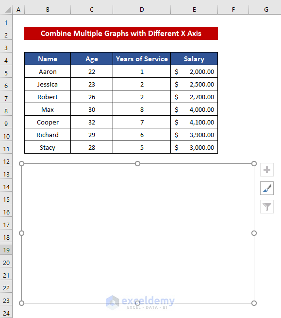
An empty graph will be displayed.
- Right-click the graph.
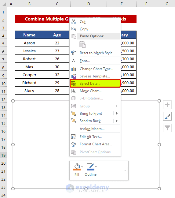
- Click Select Data.
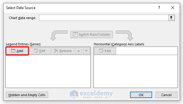
- Click Add.
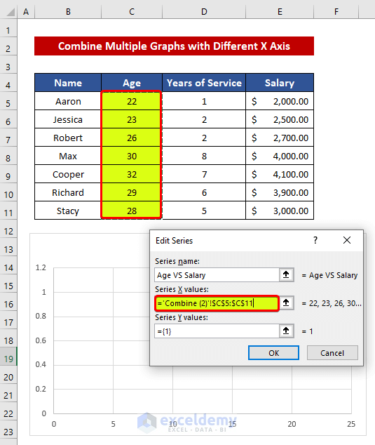
- Give your graph a title. Here, “Age VS Salary”.
- Select the series of your X values.
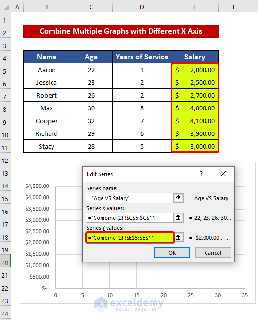
- Select the series of your Y values.
- Click OK.
2. Combine Two Graphs with Different X Axis
Steps
- Right-click the graph.
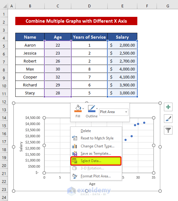
- Click Select Data.
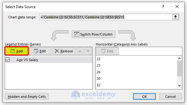
- Click Add.
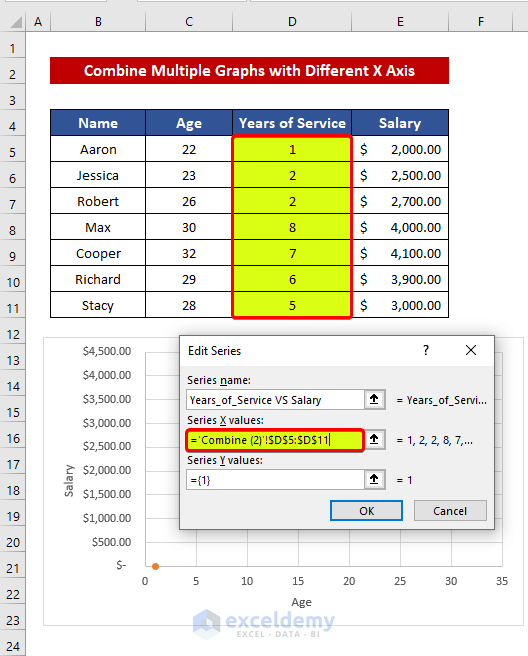
- Select the series of your X values.
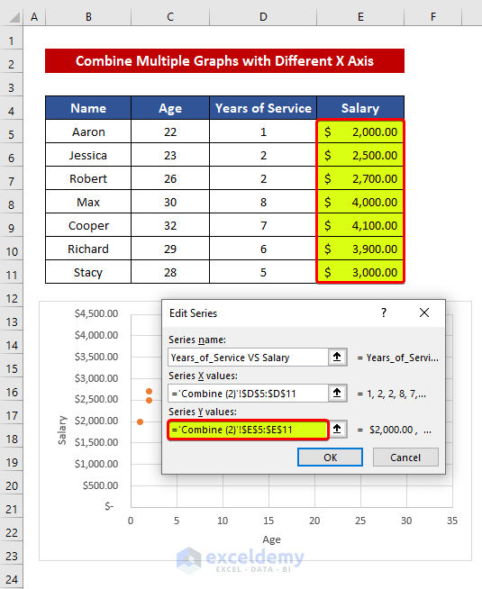
- Select the series of your Y values.
- Click OK.
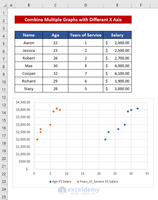
Excel labeled the two graphs with different colors.
Read More: How to Hide Secondary Axis in Excel Without Losing Data
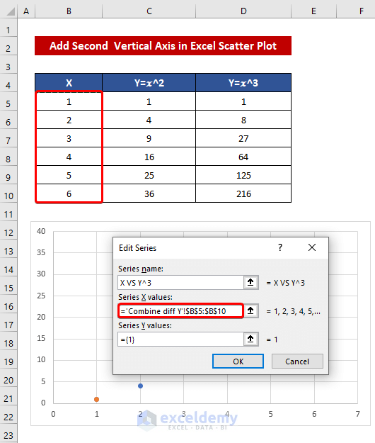
How to Add a Second or Different Vertical Axis in the Excel Scatter Plot
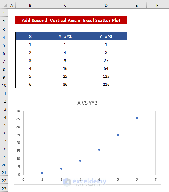
This is the dataset:
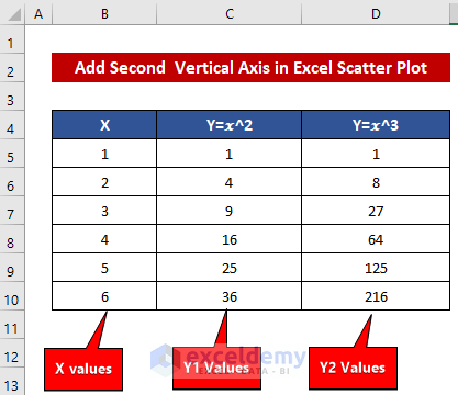
There are a series of X values. There are also two series of Y values. There are two graphs here:
- X VS Y^2
- X VS Y^3
The horizontal axis X is the same. But, we have two different Y axis.
Steps
- Go to the Insert tab.
- In Charts, click Scatter.
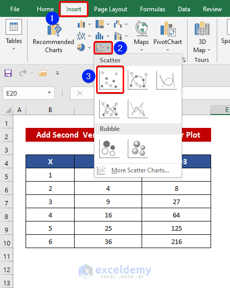
- Click Scatter.
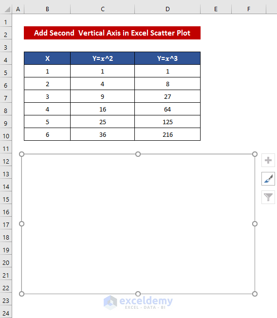
An empty graph will be displayed.
- Right-click the graph.
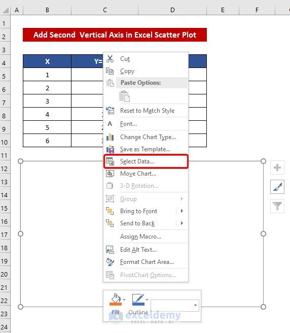
- Click Select Data.
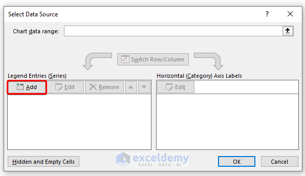
- Click Add.
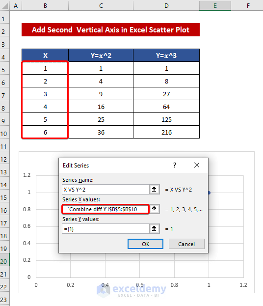
- Give your graph a title. Here, “X VS Y^2”.
- Select the series of your X values.
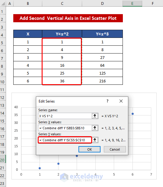
- Select the series of your Y values.
- Click OK to create the first graph.
- To add the second vertical axis, right-click the graph.

- Click Select Data.
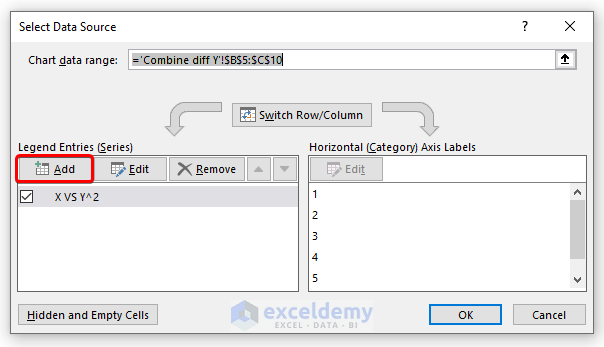
- Click Add.
- Select the series of your X values.
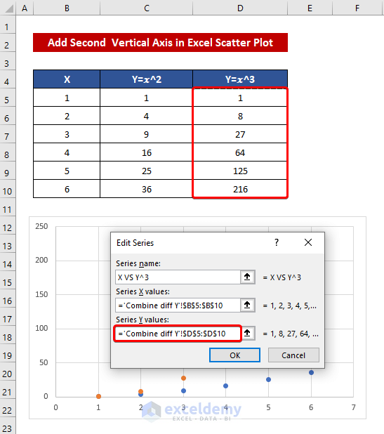
- Select the series of your Y values.
- Click OK.

The second vertical axis was added
Read More: How to Add Secondary X Axis in Excel
Download Practice Workbook
<< Go Back To Secondary Axis in Excel | Excel Charts | Learn Excel
Get FREE Advanced Excel Exercises with Solutions!
