This article will demonstrate how to add and utilize an Excel button tooltip to enhance the accessibility and user-friendliness of complex spreadsheets. In our daily professional lives, Excel button tooltip can simplify the Excel experience. They enable smooth navigation across sheets, providing additional information or instructions when users hover over buttons or shapes. This feature practically enhances the functionality of Excel and guides users effectively.
Importantly, these simple tooltips add interactivity to reports and data analysis, offering insights during sorting or filtering, triggering specific actions, and enabling contextual calculations. They contribute to making complex spreadsheets more accessible and user-friendly.

How to Create a Tooltip Button on Mouse Hover in Excel: 7 Easy Steps
In all versions of Excel, adding tooltips for buttons can be challenging. Typically, there is no built-in function specifically designed for displaying text as tooltips on command buttons. The tooltip feature in Excel is limited to certain objects such as cells, shapes, icons, images, or chart elements.
However, there is a simple way that can be used to achieve tooltips for command buttons. This article will guide you through the process and provide helpful insights.
If you require a button in Excel that serves as a cell reference, links to specific sections or sheets within a spreadsheet, and also includes a tooltip for direction and guidance, then this approach is ideal for you.
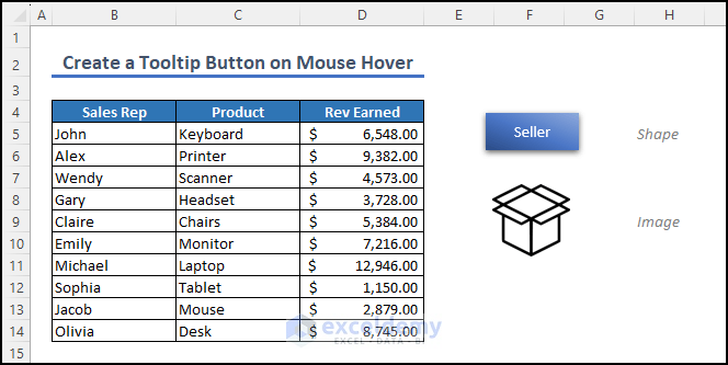
We will use the following dataset to demonstrate the process.
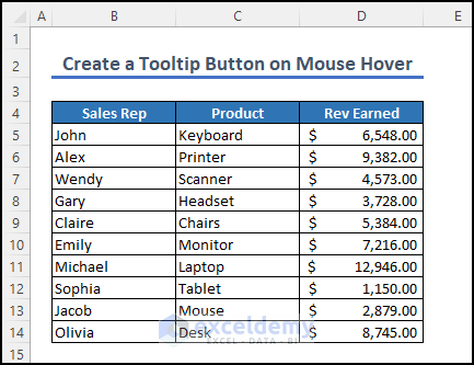
In Excel, you can use a text box, a shape, an image, or an icon as a tooltip. We will assign a shape, an image, and an icon to represent each column header: Sales Rep, Product, and Rev Earned. To make it even clearer, we will add tooltips that indicate which column each element is referring to. Check out the following steps to get insights and understand the process.
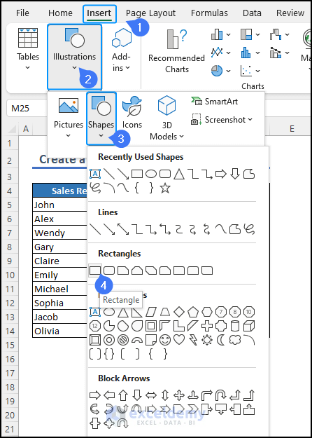
Step 1: Add Rectangle Shape as Object
To add a shape, navigate to the Insert tab and select the dropdown menu for illustrations. Choose the shapes option, and you’ll see a variety of default shapes available in Excel. Let’s select the rectangle shape for now.
Use your mouse to create any shape you prefer. Double-click on the shape or right-click and choose the edit text option to type “Seller” as the text.
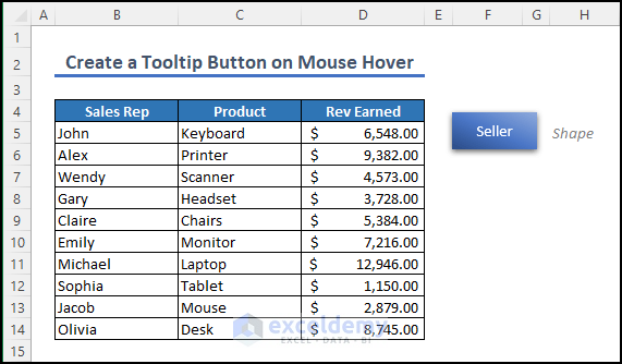
Step 2: Add Image as Object
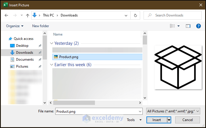
To add an image, go to the Insert tab, select Illustrations, and choose Pictures from the dropdown menu. From the Insert Picture From option, select the location where your image is stored.
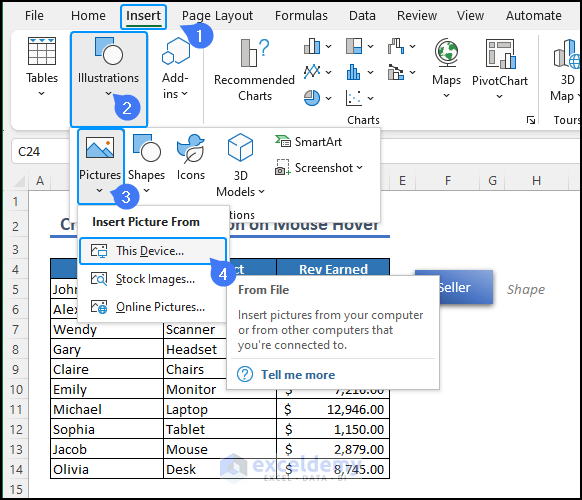
In this case, we’ll choose This Device, which opens the Insert Picture window. Select the file name and click Insert.
Step 3: Add Icons in Excel
If you want to add an icon, the process is almost identical. Go to the Insert tab, then select Illustrations and choose icons.
![]()
From the stock image window, search for an icon related to revenue and select the appropriate one from the options displayed. Click Insert to proceed.
![]()
Once again, you can use your mouse cursor to adjust the shape and size of the icon.
![]()
Step 4: Open Insert Hyperlink Window
This step is the same for each object (shape/image/icon). First, select the object and right-click on it. From the menu, choose Link.

This action will open the “Insert Hyperlink” window.
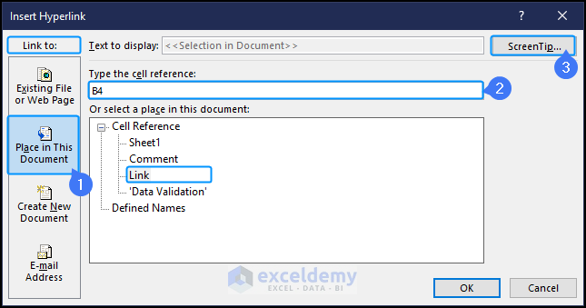
Step 5: Provide Cell Reference
From the window, select Place in This Document under the Link to the column. In the “Type the cell reference” box, enter the cell range B4 for the rectangular shape, C4 for the image, and D4 for the icon, respectively.
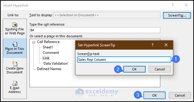
Step 6: Add Tooltips as ScreenTip Description
Next, locate the ScreenTip option in the top right corner and click on it. In the ScreenTip text field, enter the tooltip description for each object. For example, “Sales Rep column” for the shape, “Product column” for the image, and “Revenue column” for the icon Then, select OK.
Finally, click OK again in the Edit Hyperlink window to complete the process.
Step 7: Check The Result
You will notice that when you hover your mouse over each object, a tooltip will appear, providing additional information.
Furthermore, if you select the object, it will navigate you directly to the corresponding reference column.
How to Use Comment Box as a Tooltip on Mouse Hover in Excel
When collaborating with others or working in a team, one simple and effective way to provide proper direction is by using the comment box in Excel. It is user-friendly and easily accessible to all users.
Let’s consider an example where we have a dataset of sales representatives, product lists, and revenue earned. Suppose we specify that the revenue is earned in the month of January 2022. By doing so, anyone accessing the data will know that they are using all relevant information or documents for January 2022.
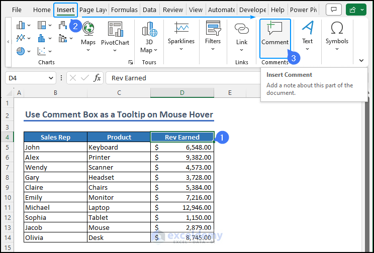
To accomplish this, first, select the cell or cell range where you want to add the tooltip. In this case, we will select cell D4, which contains the heading Rev Earned.
Next, go to the Insert tab, navigate to the Comments group, and select the Comment option.
A small window connected to the cell will appear. In the text box, type “Revenue earned in January 2022“.
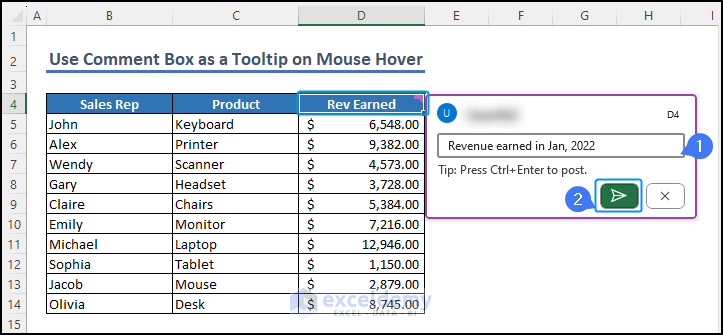
Finally, press CTRL+ENTER or click the Post Comment button with your mouse.
Now, whenever someone hovers the mouse over the header or cell D4 or selects it, the comment will appear as a helpful tooltip.
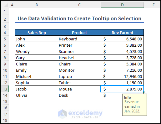
How to Use Data Validation to Create Tooltip on Selection in Excel
In Excel, you can use data validation as a tooltip to provide clear direction or relevant information. By applying data validation, Excel ensures that users follow specific guidelines or constraints when entering data. This feature actively guides users and enhances their understanding of the data being input.
To use data validation as a tooltip in Excel, follow these steps.
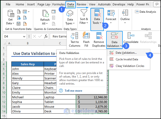
Select the cell or cell range where you want to provide tooltips. In this case, we will select the cell range C4:C14 or the Rev Earned column.
Next, go to the Data tab, and from the Data Tools group, select the Data Validation dropdown menu. Choose Data Validation from the options.
In the Data Validation window, navigate to the Input Message tab. You will find two boxes. Title and Input Message.
In the Title field, type “Info“. In the Input Message box, type “Revenue earned in January 2022“.
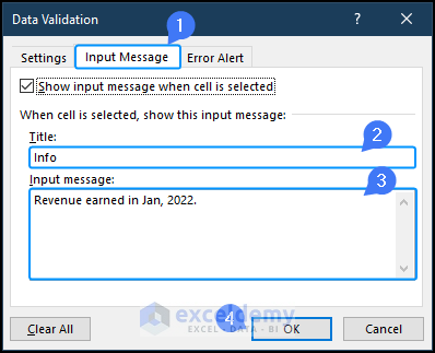
Click OK to apply the changes. Now, whenever you select any cell in the Rev earned column, the Excel button tooltip with the specified information will appear.
How to Remove Tooltip In Excel 365
Removing a tooltip in Excel 365 is a simple process. The steps may vary depending on the type of tooltip you want to remove, but they are generally simple and can be completed in just a few clicks.
If you have a comment tooltip, select the comment you wish to remove. In the top right corner of the comment box, you will see three dots. Clicking on the dots will open a menu with two options: “Delete thread” and “Resolve thread“.
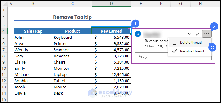
By selecting “Delete thread“, the comment tooltip will be permanently removed.
Following these steps will allow you to easily remove a comment tooltip in Excel 365.
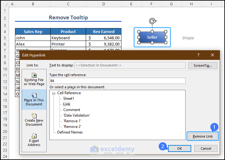
On the other hand, if you have a hyperlink tooltip that you wish to remove, navigate to the cell or object containing the hyperlink. Right-click on the cell or object to open the options menu.
From there, you can directly select the “Remove Link” option to instantly eliminate the hyperlink tooltip.
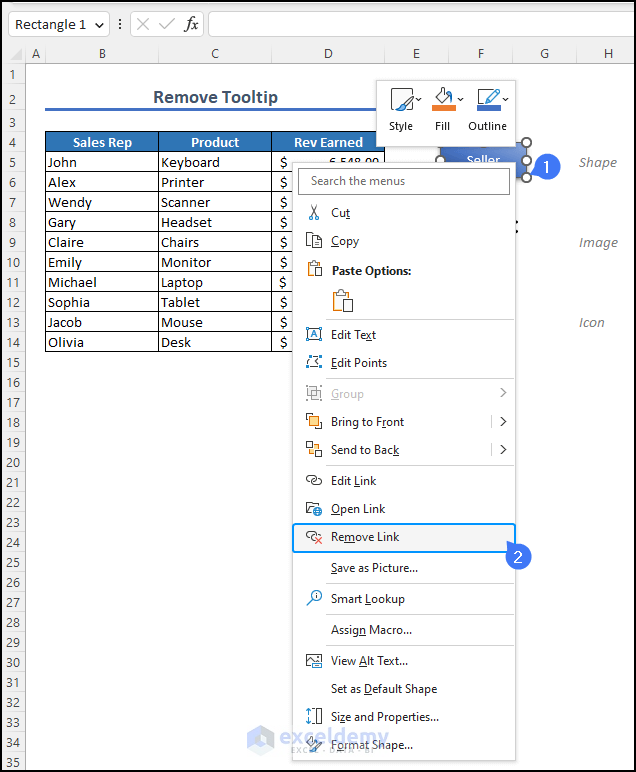
Alternatively, you can choose the “Edit Link” option, which will open the Edit Hyperlink window. In the Edit Hyperlink window, locate the “Remove Link” option at the bottom right corner and select it. This will also remove the hyperlink tooltip from your Excel 365 workbook.
Things to Remember
- Excel button tooltips are available in newer versions of Excel, such as Excel 2013 and later.
- However, the functionality of tooltips is limited to objects such as shapes, icons, images, and text boxes.
- If you use data validation as a tooltip, it will appear only when you select the cell or cell range.
Frequently Asked Questions
Q1. How do you insert a hover note in Excel?
To insert a hover note in Excel, simply right-click on the cell or object, choose “New Note“, and type your message. This will create a red mark on the cell, indicating the presence of a note. The hover note will appear as a tooltip when you hover over the cell or object, providing additional information.
Q2. Can we add a tooltip for a button?
In Excel, you can’t directly add a tooltip to a button. Instead, place a shape with a tooltip beneath the button to achieve a similar effect. When you hover the mouse over the button, it will display the tooltip from the hidden shape.
Q3. Why is a tooltip used?
Tooltips are used in Excel to provide information or instructions about buttons or objects. Additionally, They help users understand how buttons work and make the worksheet more user-friendly.
Q4. Can I customize the appearance of an Excel button tooltip?
Regrettably, Excel lacks advanced customization options for button tooltips. The tooltips usually appear as plain rectangular boxes with text. However, you have the flexibility to modify the font size and style to improve the visibility and legibility of the tooltip text.
Q5. Are button tooltips supported in all versions of Excel?
Button tooltips are not supported in all versions of Excel. The availability of button tooltips varies depending on the version of Excel you are using. Generally, newer versions of Excel, such as Excel 2013 and later, support button tooltips. Significantly, we recommend checking the specific version of Excel you are using to determine if it supports button tooltips.
Download Practice Workbook
You can download the workbook, where we have provided a practice section on the right side of each worksheet. Try it yourself.
Conclusion
Excel tooltips offer a practical solution to improve the user experience and usability of Excel spreadsheets while collaborating with others. Besides, it helps to provide directions in templates. While the built-in tooltip functionality has its limitations, there are alternative ways to incorporate tooltips using shapes, images, or data validation. It is also quite easy to add and remove tooltips in Excel.
Additionally, in our professional lives, with the help of Excel button tooltips, professionals or users can understand the functions of any button or provide additional context for data analysis, report tasking, or entering data in a sheet.
Related Articles
- How to Insert Excel Tooltip on Hover
- How to Show Full Cell Contents on Hover in Excel
- How to Edit Tooltip in Excel
- How to Create Dynamic Tooltip in Excel
- How to Create Tooltip in Excel Chart
- How to Display Tooltip on Mouseover Using VBA in Excel
- How to Add Tooltip to UDF in Excel
<< Go Back to Excel Tooltip | Learn Excel
Get FREE Advanced Excel Exercises with Solutions!
