How to Create Dynamic Tooltip in Excel (with Easy Steps)

Microsoft Excel is one of the best programs you can use right now. With the tools and features that Excel offers, you can do an infinite number of things with a dataset. We have to make tooltips for several cells in Excel regularly because they tell us something about the data in the cell. This post will talk about step-by-step procedures to make tooltips. You should check out this easiest way to make a Dynamic Tooltip in Excel.

How to Create Dynamic Tooltip in Excel: with Easy Steps

We will look at a sample dataset as an example. For example, the dataset below has columns for Name, Date of Birth, and Age. We’ll use this dataset to create a dynamic tooltip in Excel.

We are using Microsoft Excel 365 to demonstrate this tutorial. You are free to choose the edition that works best for you.

Step 01: Use Formula to Fetch Data from Another Sheet

• In a new worksheet, create a data table with columns S.L No and Name. In the first column, input the serial number like 1,2,3, etc. And in the second column, write names in a random serial from the names of the Dataset worksheet.
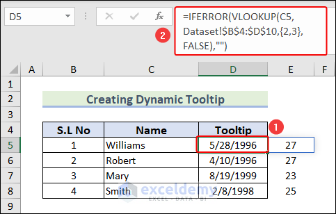
• Create a Tooltip column under Column D. Here, write the following formula in cell D5.

The VLOOKUP function returns the value of the same row from the specified column of the given table, where the value in the leftmost column matches the lookup_value.

• Then, use the Fill Handle tool to AutoComplete the output in the remaining cells.

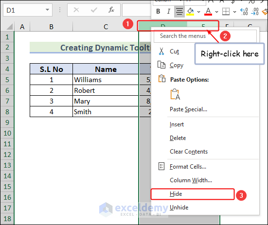
• Now, select columns D and E and right-click on the mouse. From the context menu, click on the Hide option to hide these two columns.

Step 02: Assign VBA Code

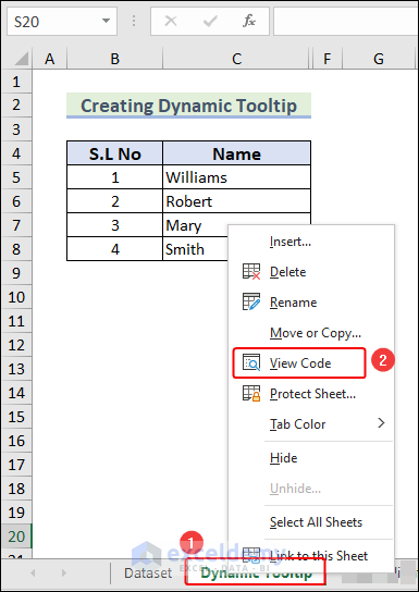
• Right-click on the sheet name tab and click on View Code on the context menu.

• Paste the following VBA code in the code module specified for this particular worksheet.

Private Sub Worksheet_SelectionChange(ByVal Target As Range)
Dim rng As Range
Dim cell As Range

' Clear existing comments
For Each rng In Me.UsedRange
If Not rng.Comment Is Nothing Then
rng.Comment.Delete
End If
Next rng

If Target.Count > 1 Then Exit Sub
If Target.Column <> 3 Then Exit Sub
If Target.Row < 5 Then Exit Sub

Dim tooltipText As String
tooltipText = "Birth Date: " & Target.Offset(0, 1).Value & _
vbCrLf & "Age: " & Target.Offset(0, 2).Value

Target.AddComment tooltipText ' Add comment with tooltip text
Target.Comment.Shape.TextFrame.AutoSize = True ' Adjust the _
comment box size automatically
End Sub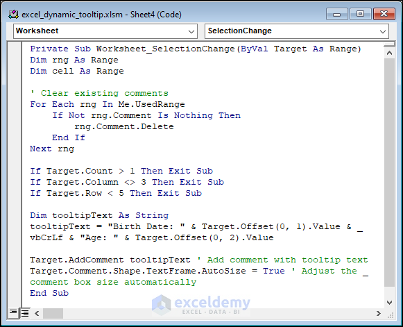

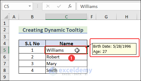
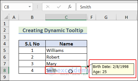
• Now, return to the worksheet. Click on any cell of the Name column, and it’ll show the tooltip with the person’s Birth Date, and Age. So, it’s dynamic.

• The same happens for any other cell in this column.

3 Methods to Create Static Tooltip in Excel

The first method in this article shows how to use the Data Validation Feature to create a tooltip. On the other hand, two more ways to generate tooltips using Excel VBA and the Link Option.

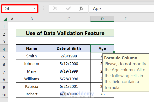
1. Utilize Data Validation Feature to Generate Static Tooltip

A feature known as data validation enables you to establish guidelines dictating the kind of data we may enter into specific cells of your sheet. In this case, we will use the Data Validation feature to make a static tooltip for cell D4 in the current sheet. Please pay close attention to these instructions if you want to work well on the assignment.

📌 Steps:

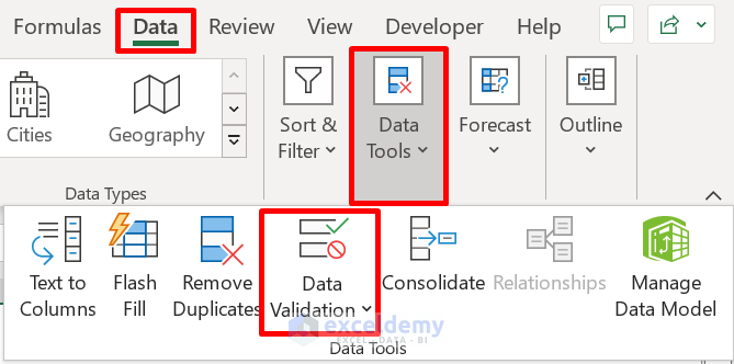
• First, navigate to the Data tab.
• Second, choose Data Tools from the Data Tools group.
• After that, click the Data Validation icon.

• Subsequently, the Data Validation window will open.
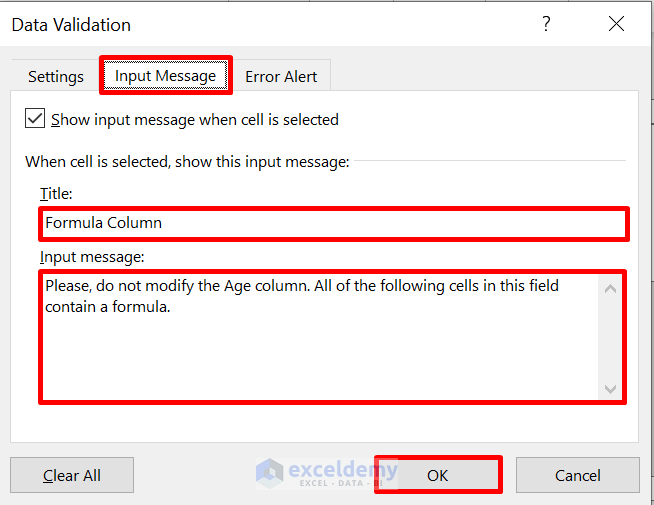
• Later, go to Input Message.
• At this point, type the tooltip title in the Title section.
• Next, write a message in the Input Message box.
• Now, hit OK.

• Presently, select cell D4.
• Consequently, it will produce the intended output as below.

2. Create Tooltip Using Excel VBA

VBA is the name for Visual Basic for Applications. VBA is a programming language that Microsoft made. Users can use the programming language VBA to get to capabilities that Excel doesn’t support. In this part, we’ll use VBA to make tooltips that are always up-to-date. Please do the assignment by following the steps below.

📌 Steps:

• To begin, choose the working sheet as the active sheet.
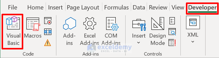
• Latterly, go to the Developer tab.
• Second, from the Code group, pick Visual Basic.

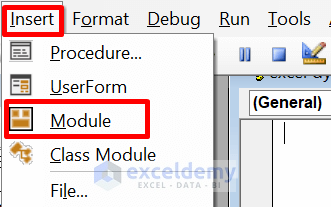
• After that, click Insert followed by Module to get a Module Box.

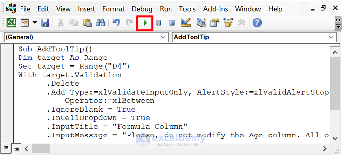
• Next, type the formula below in the Module Box.

Sub AddToolTip()
Dim target As Range
Set target = Range("D4")
With target.Validation
      .Delete
      .Add Type:=xlValidateInputOnly, AlertStyle:=xlValidAlertStop, _
          Operator:=xlBetween
      .IgnoreBlank = True
      .InCellDropdown = True
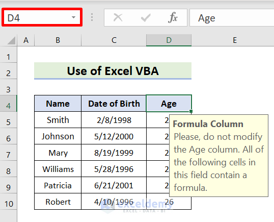
      .InputTitle = "Formula Column"
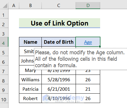
      .InputMessage = "Please, do not modify the Age column. All of the following cells in this field contain a formula."
      .ShowError = True
  End With
End Sub

• Later, press F5 or click the Run button.

• Then, select the D4 cell.
• As a result, we will get the output below.

Read More: How to Display Tooltip on Mouseover Using VBA in Excel

3. Apply Link Option to Create Static Tooltip

Utilizing the Link Option is an additional fun and fascinating approach to creating a tooltip. In this part of the tutorial, we will use the Link option to generate a tooltip. To complete the task, please follow the steps that are listed below.

📌 Steps:

• First, pick the D4 cell of the working sheet.
• Second, right-click in D4.
• Subsequently, the Context bar will pop up.

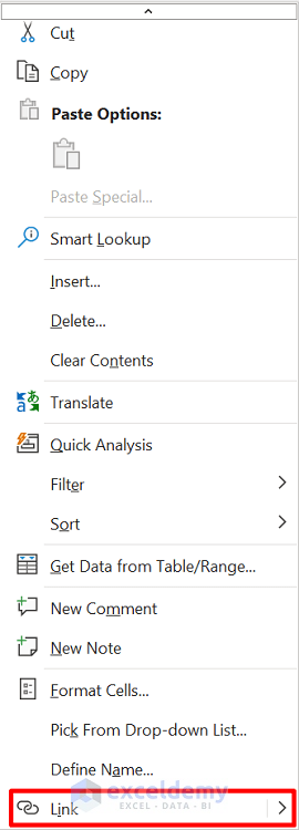
• Latterly, choose the Link option.
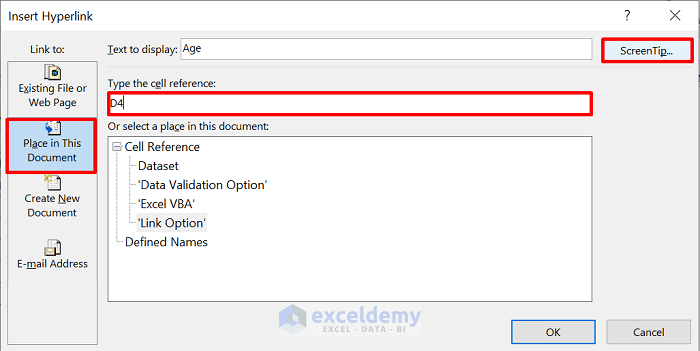
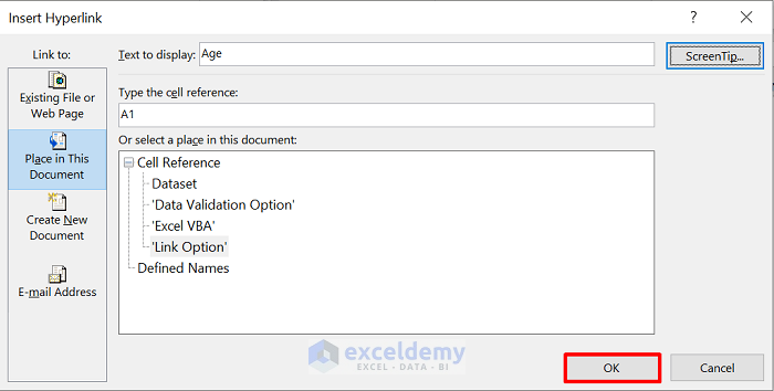
• Due to this, the Insert Hyperlink window will open.
• Now, click the Place in This Document icon from the Link To section.
• Then, type D4 in the Type The Cell Reference box.
• After that, go to ScreenTip.

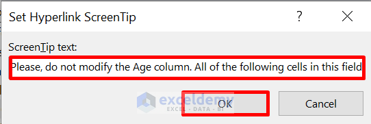
• Consequently, the Set Hyperlink ScreenTip window will come up.
• Presently, write a message in the ScreenTip Text box.
• Later, hit OK.

• Now, go to the Insert Hyperlink window again and click the OK button.

• At this point, use the Mouse cursor to hover over cell D4.
• Finally, we will get the desired output like the one below.

Read More: How to Add Tooltip to UDF in Excel

Download Practice Workbook

You may download a free copy of the example workbook we mentioned during the presentation by clicking on the link below.

Conclusion

After this point, you can build a Dynamic Tooltip in Excel by following the methods we covered. Be sure to let us know if you come up with any other strategies to get the job done or if you have any fresh ideas. Remember to ask questions, comment, or provide recommendations in part down below.

Related Articles

• How to Edit Tooltip in Excel
• How to Create Tooltip in Excel Chart
• How to Remove Tooltip in Excel
• How to Show Full Cell Contents on Hover in Excel
• How to Insert Excel Tooltip on Hover
• Excel Button Tooltip

<< Go Back to Excel Tooltip | Learn Excel