How to Create a Tooltip in an Excel Chart (Easy Steps)

What is a Tooltip?

Tooltip is a message or note that appears when the mouse pointer rests on an icon or any graphical interface. In Microsoft Excel, you can put a chart tooltip on a cell. Whenever you hover the mouse pointer over the selected cell, the animation of that chart appears to you as a tooltip.

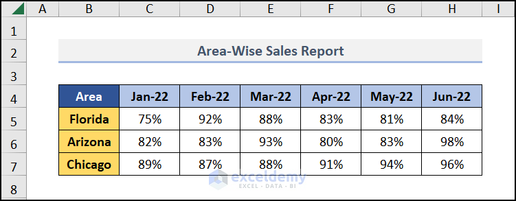
Dataset Overview

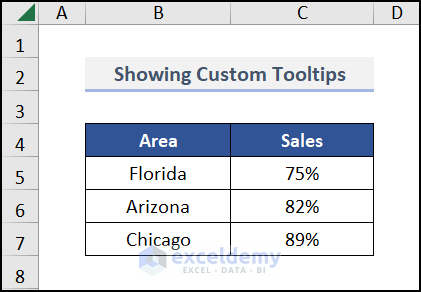
To demonstrate the steps, we’ll us a dataset of Area-wise Sales Reports for 6 months.

Step 1 – Input Raw Data

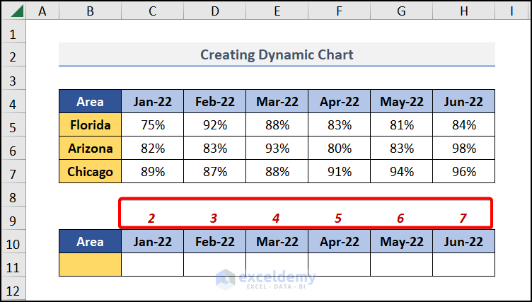
• Enter your raw data for creating the dynamic chart. We’ll use Area-Wise’s Sales Report dataset for 6 months.
• Create a serial number for the Month column (see the image).

• In cell C11, insert the following formula:

Here,

• • $B$11 is the lookup value (e.g., the selected Area).
  • The function searches for this value in the table array $B$4:$H$7.
  • Set the col_index_num to cell C$9 and range_lookup to 0.
  • This function retrieves the corresponding Sales value based on the selected Area.

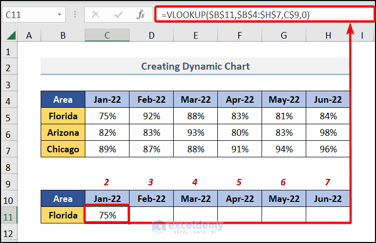
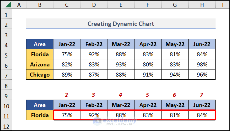
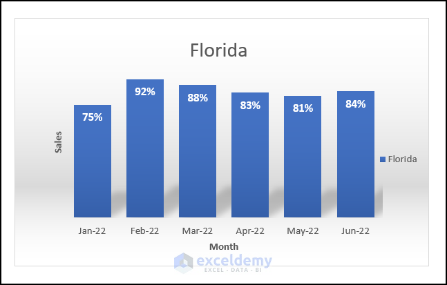
The Sales value of Florida has been added. If the Area in B11 is changed, the values will be changed.

Step 2 – Create a Chart

• Select the entire dataset from B10:H11.
• Navigate to the Insert tab, choose Insert Column or Bar Chart, and pick Clustered Column.

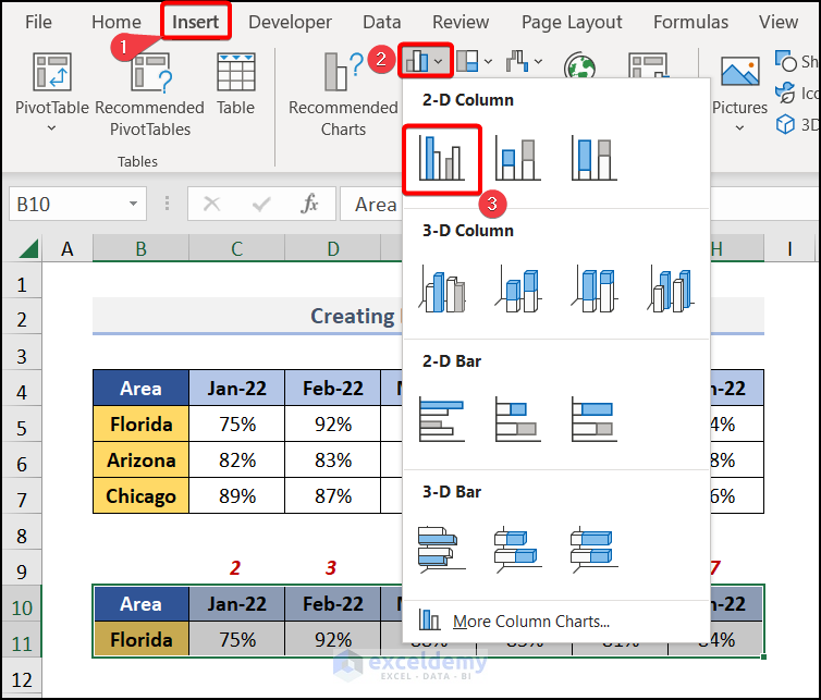
• Customize your chart by adding Axis Titles and selecting a suitable style from Chart Styles.

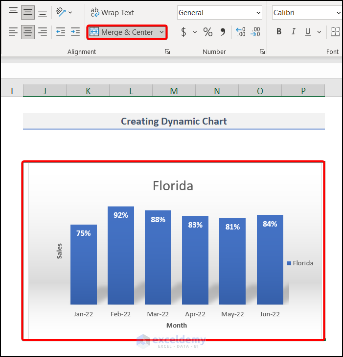
• Select the chart cells and choose the Merge & Center command in the Alignment section from the Home tab.

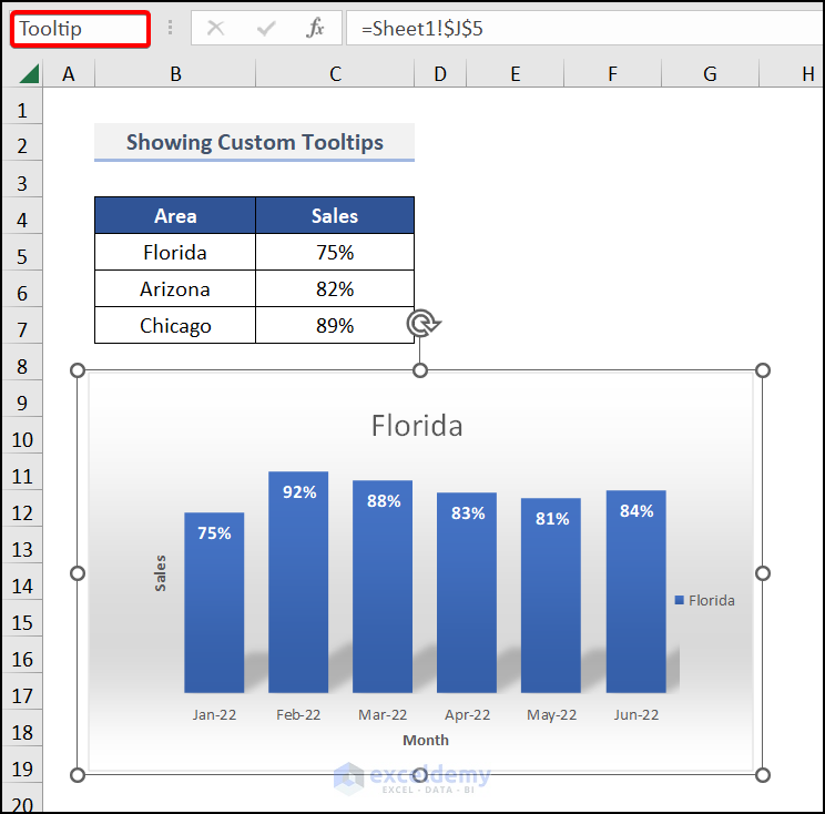
Step 3 – Paste Chart as Linked Picture

• Copy the chart (CTRL + C).
• Move to another sheet where you want to add the tooltip.
• Under the Home tab, select the Paste dropdown in the Clipboard group, and choose Linked Picture.

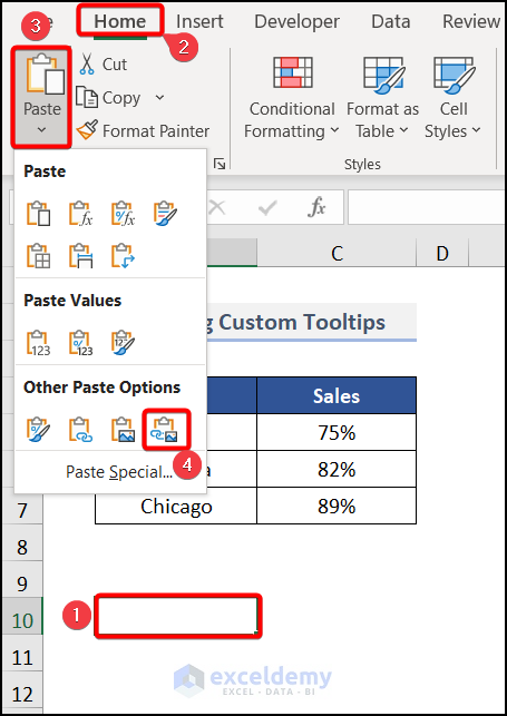
• Name the picture Tooltip.

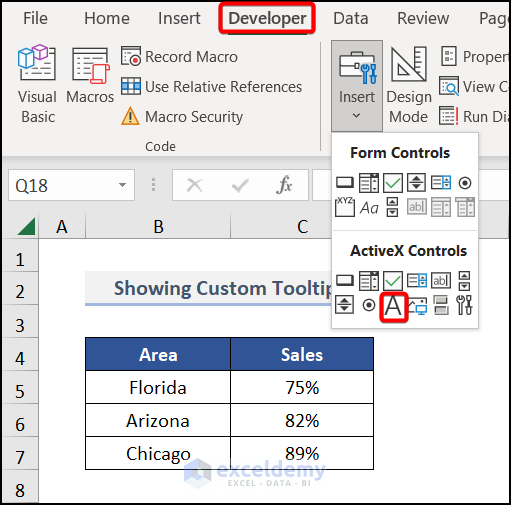
Step 4 – Add Labels

• In the Developer tab, choose the Insert dropdown in the Controls section and select Label.

• Label the Area and Sales as needed.

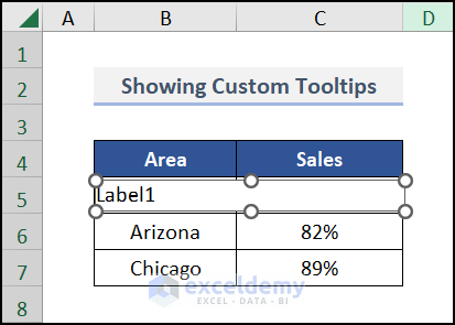
• Copy Label 1 and paste it for other cells.

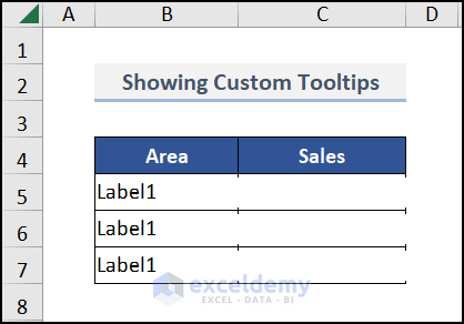
Step 5 – Customize Labels

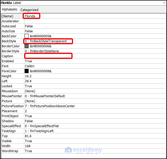
• Select any Label, go to Properties in the Controls section.

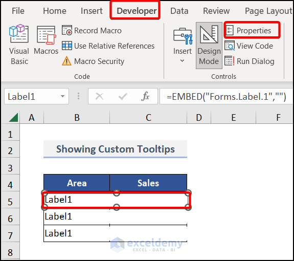
• Customize the label appearance (e.g., change the Name, make BackStyle Transparent, leave Caption blank).

The tooltip should look similar to the image below.

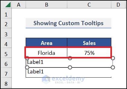
• Apply the same steps for the other Labels.

Read More: How to Edit Tooltip in Excel

Step 6 – Employ VBA Code

• Exit Design Mode in the Controls ribbon group.
• Navigate to the Developer tab and choose Visual Basic.

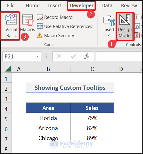
• In the Visual Basic editor, choose the Insert tab, then select Module to create a new module (e.g., Module 1).

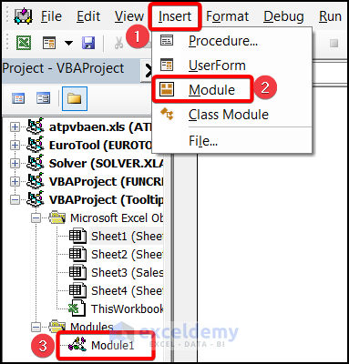
• Enter the VBA code in this module.

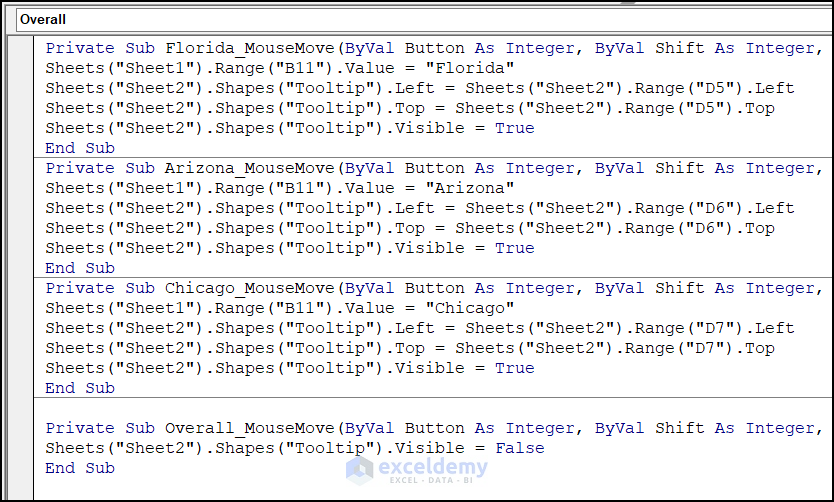
Private Sub Florida_MouseMove(ByVal Button As Integer, ByVal Shift As Integer, ByVal X As Single, ByVal Y As Single)
Sheets("Sheet1").Range("B11").Value = "Florida"
Sheets("Sheet2").Shapes("Tooltip").Left = Sheets("Sheet2").Range("D5").Left
Sheets("Sheet2").Shapes("Tooltip").Top = Sheets("Sheet2").Range("D5").Top
Sheets("Sheet2").Shapes("Tooltip").Visible = True
End Sub
Private Sub Arizona_MouseMove(ByVal Button As Integer, ByVal Shift As Integer, ByVal X As Single, ByVal Y As Single)
Sheets("Sheet1").Range("B11").Value = "Arizona"
Sheets("Sheet2").Shapes("Tooltip").Left = Sheets("Sheet2").Range("D6").Left
Sheets("Sheet2").Shapes("Tooltip").Top =Sheets("Sheet2").Range("D6").Top
Sheets("Sheet2").Shapes("Tooltip").Visible = True
End Sub
Private Sub Chicago_MouseMove(ByVal Button As Integer, ByVal Shift As Integer, ByVal X As Single, ByVal Y As Single)
Sheets("Sheet1").Range("B11").Value = "Chicago"
Sheets("Sheet2").Shapes("Tooltip").Left = Sheets("Sheet2").Range("D7").Left
Sheets("Sheet2").Shapes("Tooltip").Top = Sheets("Sheet2").Range("D7").Top
Sheets("Sheet2").Shapes("Tooltip").Visible = True
End Sub
Private Sub Overall_MouseMove(ByVal Button As Integer, ByVal Shift As Integer, ByVal X As Single, ByVal Y As Single)
Sheets("Sheet2").Shapes("Tooltip").Visible = False
End Sub

• Press F5 to run the code.
• Go to Sheet2 and hover the mouse over an Area to see the tooltip in action.

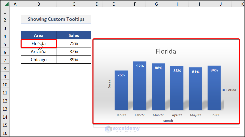
We have added a GIF to help you understand how the tooltip works.

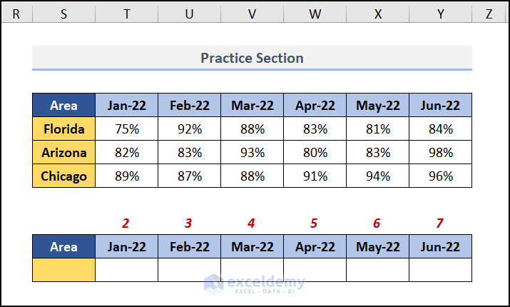
Practice Section

We have provided a practice section on each sheet on the right side for your practice.

Download Practice Workbook

You can download the practice workbook from here:

Related Articles

• How to Create Dynamic Tooltip in Excel
• How to Remove Tooltip in Excel
• How to Show Full Cell Contents on Hover in Excel
• How to Insert Excel Tooltip on Hover
• Excel Button Tooltip
• How to Display Tooltip on Mouseover Using VBA in Excel

<< Go Back to Excel Tooltip | Learn Excel