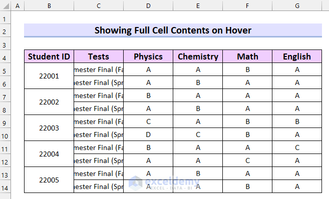
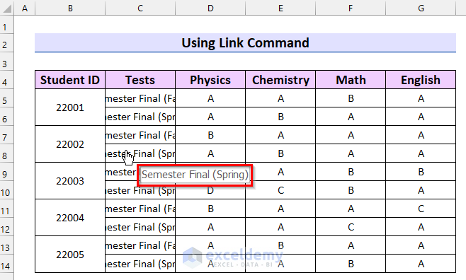
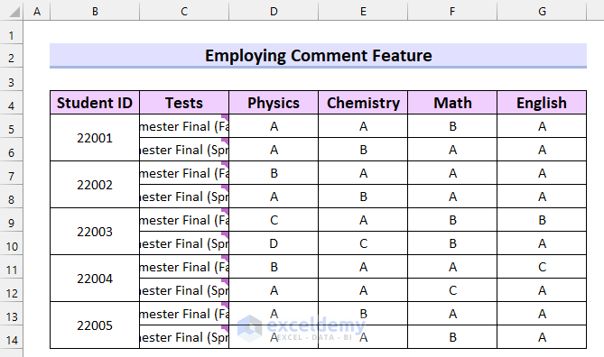
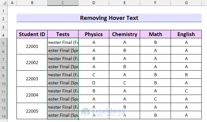
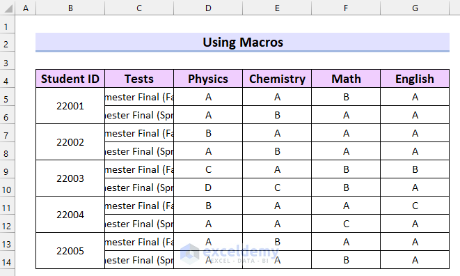
How to Show Full Cell Contents on Hover in Excel (5 Quick Ways)

The sample dataset contains the grades of 5 students in 4 subjects on different tests. The full cell contents for the column named Tests is not visible.

Method 1 – Using Link Command to Show Full Cell Contents on Hover in Excel

Steps:

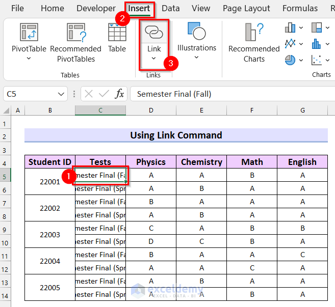
Select the cell where you want to show the contents on hover. Here C5 is selected.
Go to the Insert tab.
Select Link.

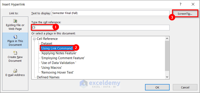
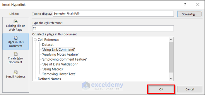
A dialog box named Insert Hyperlink will appear.

Enter the cell address selected in the Type the cell reference section.
Select the worksheet.
Select ScreenTip.

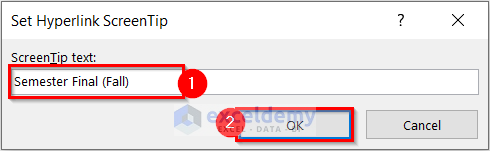
The Set Hyperlink ScreenTip dialog box will appear.

Enter the full contents of the cell as ScreenTip text.
Click OK.

Select OK on the Insert Hyperlink screen.

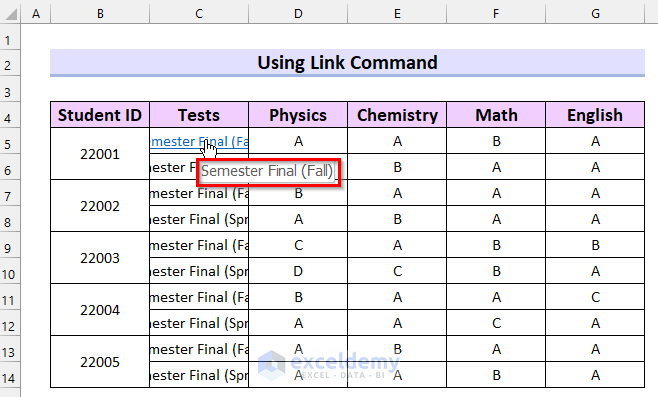
A link has been inserted and if you hover your mouse cursor over the cell the full contents of the cell are showing.

Insert hyperlinks to the other cells in the same way.

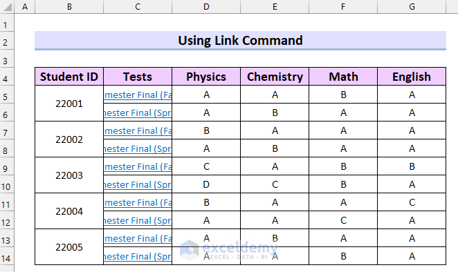
The link format should be removed and changed to a normal font.

Select the cells that need to be changed.
Right-click on the selected cell range.
Select Format Cells.

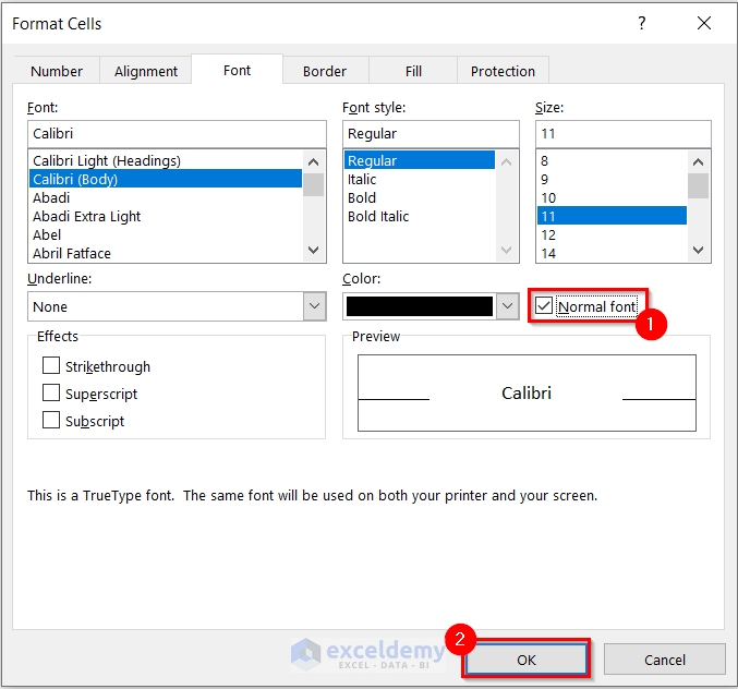
The Format Cells dialog box will appear.

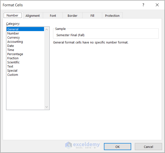
Go to the Font tab.
Check the Normal Font box.
Select OK.

The hyperlinks have changed to the normal font but hovering over the cell will reveal the full cell contents.

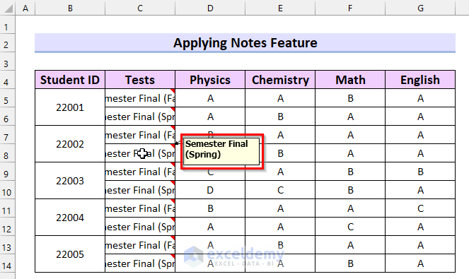
Method 2 – Applying Notes Feature to Show Full Cell Contents on Hover in Excel

Steps:

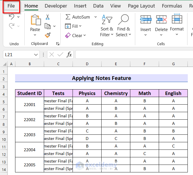
Go to the File tab.

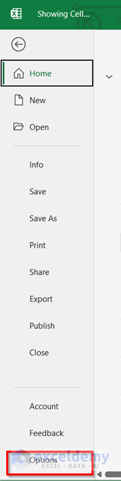
Select the Options.

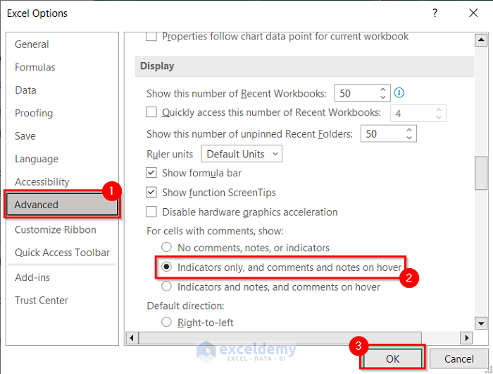
A dialog box named Excel Options will appear.

Select the Advanced tab.
Select the Indicators only, and comments and notes on hover option.
Select OK.

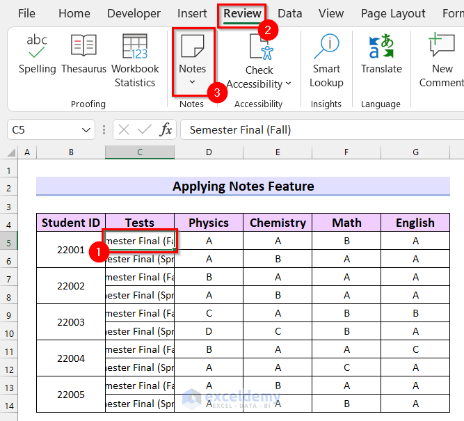
Select the cell where you want to show the full cell contents.
Go to the Review tab.
Select Notes.

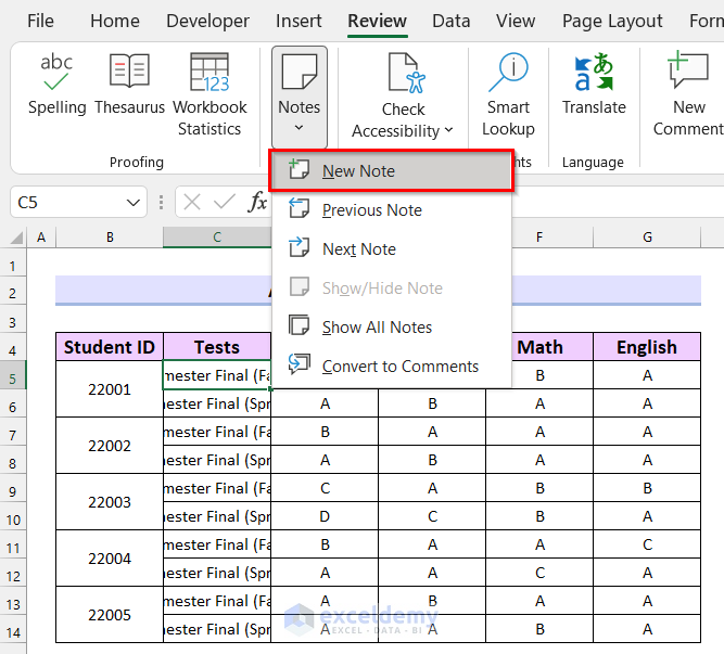
A drop-down menu will appear.

Select New Note from the drop-down menu.

A note will be added to the selected cell.

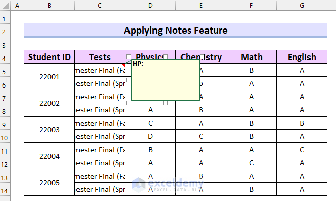
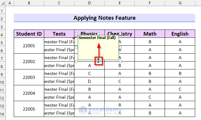
Enter the full cell contents of the selected cell as a note.
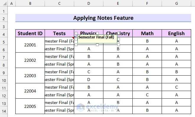
The notes size can be changed by selecting and dragging the border of the note box.

Select any cell to hide the note. The red triangle in the corner of the cell indicates there is a note present.

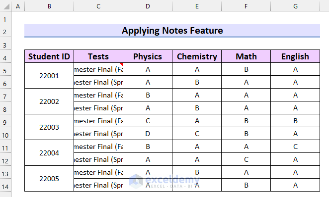
Add notes to all the other cells.

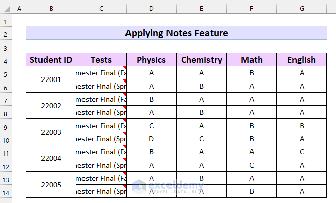
Hover overing any cell will show the full contents of the cell as a note.

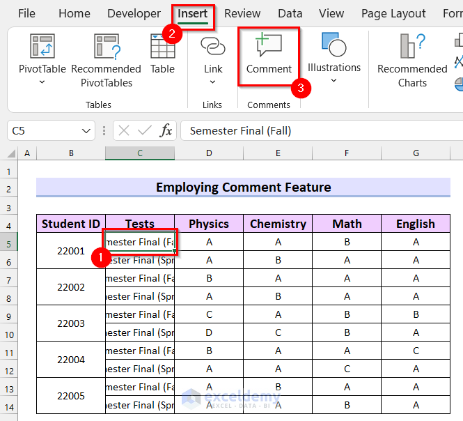
Method 3 – Employing Comment Feature in Excel

Steps:

Select the cell where you want to show the full cell contents on hover.
Go to the Insert tab.
Select Comment.

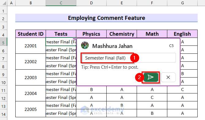
A comment box will appear.

Enter the full cell contents in the comment box.
Select the Send button to add the comment.

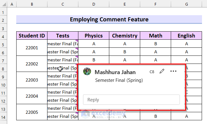
A comment has been added to the cell which is illustrated by the purple mark on the corner of the cell.

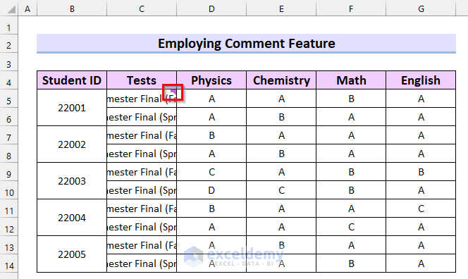
Add comments to all the other cells.

The full cell contents are visible in the comment box when hovering the mouse over the cell.

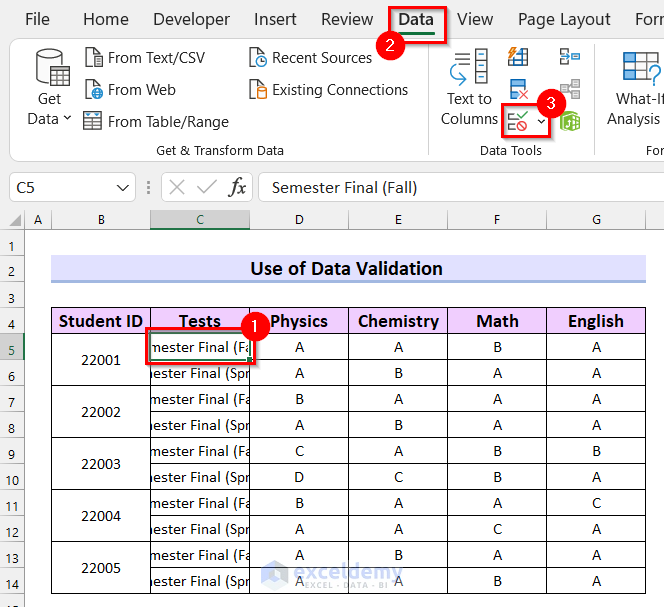
Method 4 – Use of Data Validation in Excel

Steps:

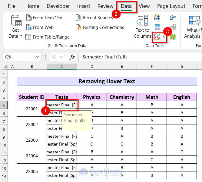
Select the cell where you want to show the full cell contents on hover.
Go to the Data tab.
Select Data Validation.

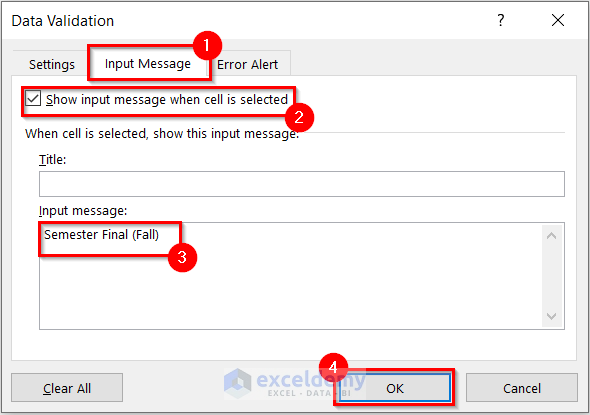
A dialog box named Data Validation will appear.

Select the Input Message tab.
Check the Show input message when cell is selected option.
In the Input message enter the full cell contents.
Select OK.

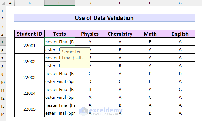
You will be able to see full cell contents on a message box when the cell is selected.

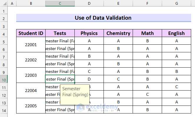
Add message boxes to all the other cells. You will be able to see the full cell contents in a message box when a cell is selected.

Method 5 – Using Macros to Show Full Cell Contents on Hover

Steps:

Go to the Developer tab.
Select Visual Basic.

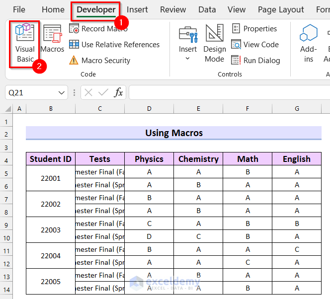
The Visual Basic window will open.

Select the Insert tab.
Select Module.

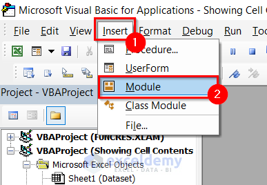
A module will open.

Enter the following code in the module.

Sub Hover_Text()
    Dim row_no As Integer
    For row_no = 5 To 14
         With Cells(row_no, 3)
                If ActiveSheet.Cells(row_no, 3).Value <> "" Then
                    .ClearComments
                    .AddComment
                    .Comment.Visible = False
                    .Comment.Text Text:=Cells(row_no, 3).Value
                    .Comment.Shape.ScaleWidth 1, msoFalse, msoScaleFromTopLeft
                    .Comment.Shape.ScaleHeight 0.5, msoFalse, msoScaleFromTopLeft
                End If
            End With
        Next
End Sub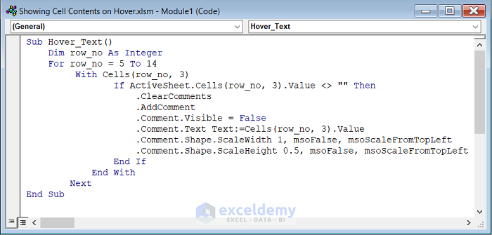

Code Breakdown

A Sub Procedure named Hover_text is created. A variable named row_no as Integer is declared. For Next Loop runs the Sub Procedure through the cells selected. The With Statement skips requalifying the name of the object. IF Statement checks if the cell is non-empty. If the cell is non-empty then the code will clear the existing comments at first by using the ClearComments method. The AddComment Method adds comments to the cells. The code will show the value in the selected cell as a Comment. The Height and Width of the comment box are declared. The IF Statement ends. The With Statement ends. The Sub Procedure ends.

Save the code and go back to your worksheet.

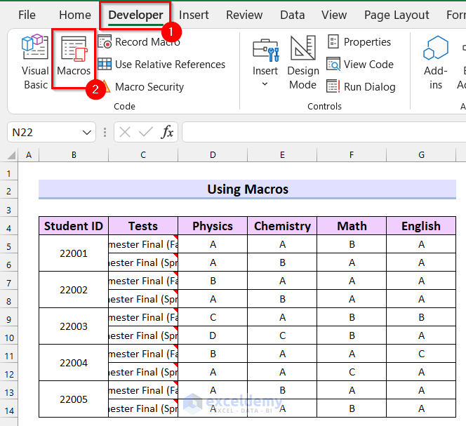
Go to the Developer tab.
Select Macros.

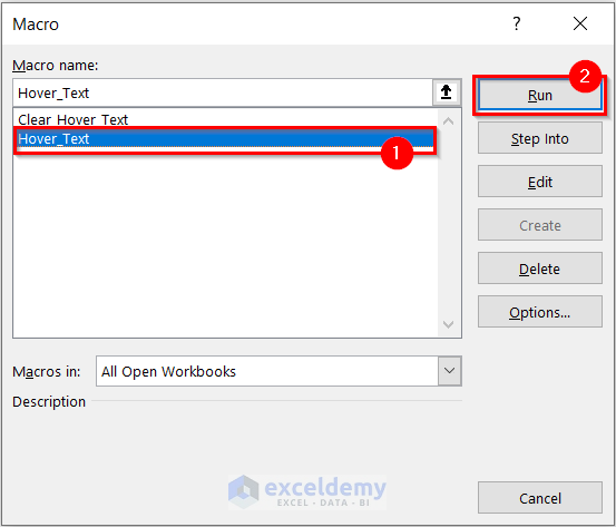
The Macro dialog box will appear.

Select Hover_Text as the Macro name.
Select Run.

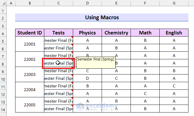
The full cell contents are visible as a comment if you hover on a cell.

How to Remove Hover Text in Excel

Steps:

Select the cells where you added the hyperlinks to show the full cell contents on hover.

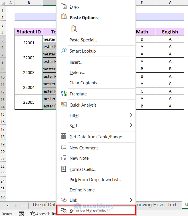
Right-click on the selected cells.
Select Remove Hyperlinks.

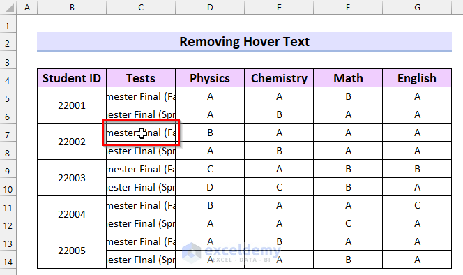
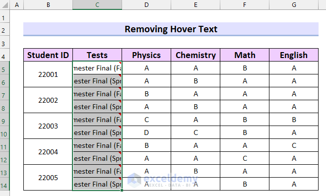
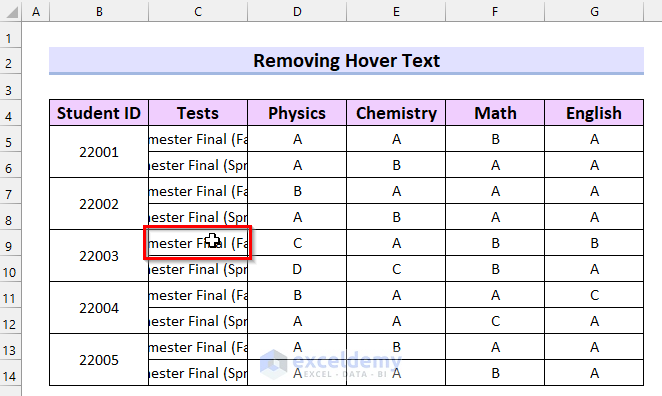
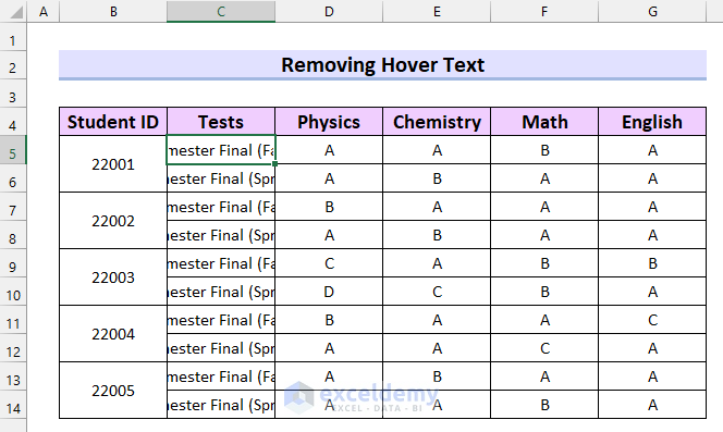
The full cell contents are not showing anymore.

How to remove the hover texts by applying the Notes feature.

Select the cells that contain the hover text.

Right-click on the selected cells.
Select Delete Note.

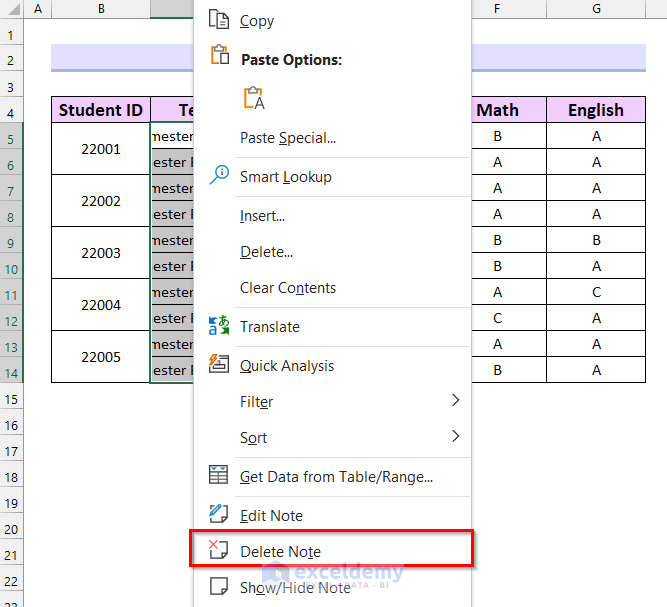
The hover text no longer appears.

How to remove the hover texts by applying the Comments feature.

Select the cells with comments.

Right-click on the selected cells.
Select Delete Comment.

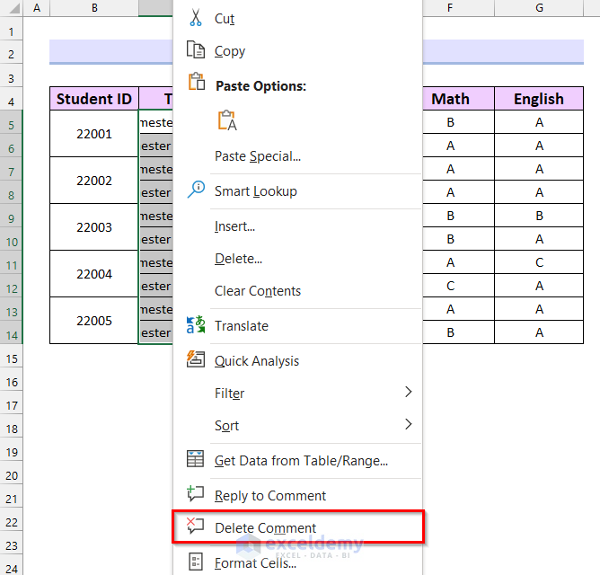
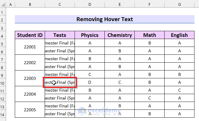
The full cell contents are not showing anymore.

How to remove the hover texts by applying the Data Validation feature.

Select the relevant cell.
Go to the Data tab.
Select Data Validation.

The Data Validation dialog box will appear.

Select the Input Message tab.
Uncheck the Show input message when cell is selected option.
Select OK.

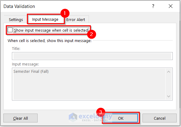
The full cell contents are not showing anymore.

How to use VBA Code to remove Hover text.

Select the Insert tab.
Select Module.

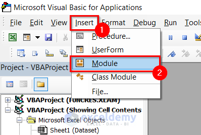
A module will open.

Enter the following code in the module.

Sub Clear_Hover_Text()
    Dim row_no As Integer
    For row_no = 5 To 14
        ActiveSheet.Cells(row_no, 3).ClearComments
    Next
End Sub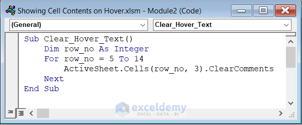

Code Breakdown

A Sub Procedure named Clear_Hover_Text is created. A variable named row_no as Integer is declared. A For Next Loop runs the Sub Procedure through the selected column. The ActiveSheet property selects the cells from the current sheet and ClearComments method removes the comments from the cells. The Sub Procedure ends.

Save the code and go back to the worksheet.

Go to the Developer Tab.
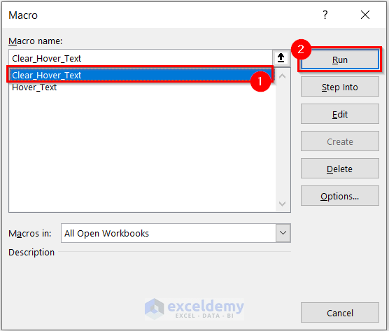
Select Macros.

The Macros dialog box will appear.

Select Clear_Hover_Text as the Macro name.
Select Run.

The full cell contents are not showing anymore.

Practice Section

Download Practice Workbook

Showing Cell Contents on Hover.xlsm

<< Go Back to Excel Tooltip | Learn Excel

Get FREE Advanced Excel Exercises with Solutions!

How to Show Full Cell Contents on Hover in Excel (5 Quick Ways)

Method 1 – Using Link Command to Show Full Cell Contents on Hover in Excel

Method 2 – Applying Notes Feature to Show Full Cell Contents on Hover in Excel

Method 3 – Employing Comment Feature in Excel

Method 4 – Use of Data Validation in Excel

Method 5 – Using Macros to Show Full Cell Contents on Hover

How to Remove Hover Text in Excel

How to remove the hover texts by applying the Notes feature.

How to remove the hover texts by applying the Comments feature.

How to remove the hover texts by applying the Data Validation feature.

How to use VBA Code to remove Hover text.

Practice Section

Related Articles

Leave a Reply Cancel reply