Concatenate means to merge or combine two or more cells’ contents into a single cell.
Method 1 – Applying Ampersand(&) Operator to Concatenate Rows in Excel
You can concatenate strings using Ampersand (&). The advantage of using the Ampersand operator is that there is no limit for allowable strings to join.
Steps:
- Type the below formula in Cell C5.
=B5&" "&B6&" "&B7&" "&B8&" "&B9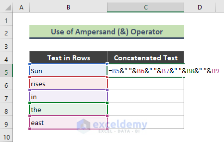
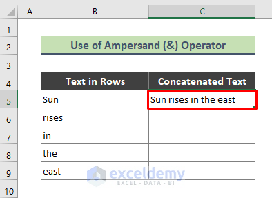
- Hit Enter and the texts from 5 rows are joined.
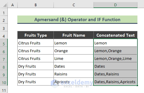
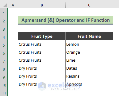
Method 2 – Using Excel IF Function and ‘&’ Operator to Concatenate Rows
The IF function can be used in conjunction with the ‘&’ operator to concatenate rows. The sample dataset contains the fruits type in column B and related fruit names are listed in column C.

Steps:
- Type the below formula in Cell D5 and hit Enter.
=IF(B5=B4,D4&","&C5,C5)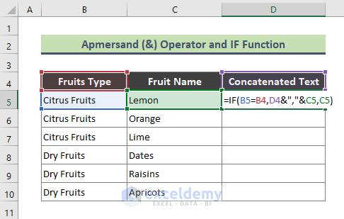
- Use the Fill Handle (+) tool to copy the formula to the range D5:D10.
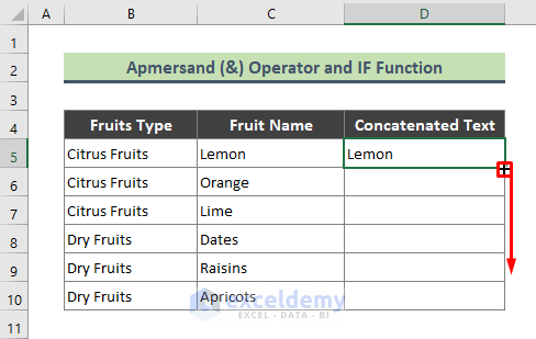
- A growing list of fruit names to their corresponding fruit type is returned.
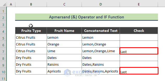
- This is not the final result. As the dataset is sorted alphabetically according to fruit type, the cell containing the most text will be the desired result.
- To find the cell with the most text, type the below formula in Cell E5.
=IF(B5<>B6,"Last","")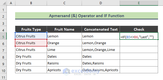
- Press Enter and use the Fill Handle tool to copy the formula to the rest of the cells which returns the below result; ‘Last’ is assigned to the longest concatenated texts.
Related Content: How to Combine Multiple Rows into One Cell in Excel
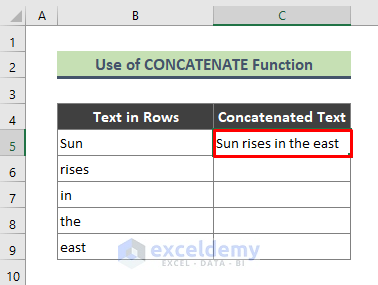
Method 3 – Inserting Excel CONCATENATE Function to Combine Rows
Use the CONCATENATE function to join excel rows.
Steps:
- Type the following formula in Cell C5.
=CONCATENATE(B5," ",B6," ",B7," ",B8," ",B9)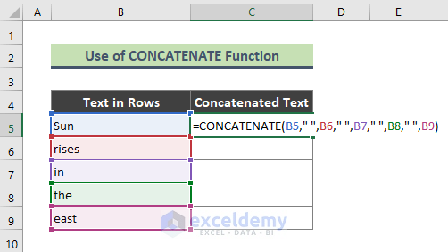
- Press Enter.
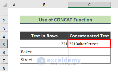
Method 4 – Using CONCAT Function to Combine Rows in Excel
In Excel 365 and Excel 2019, you can use the CONCAT function to combine text from a range spread over different rows.
Steps:
- Type the below formula in Cell C5 to join text from the range B5:B7.
=CONCAT(B5:B7)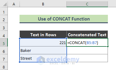
- Press Enter.
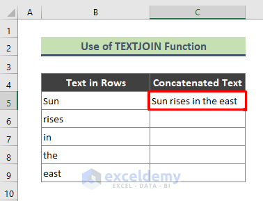
Method 5 – Applying Excel TEXTJOIN Function to Join Rows
Steps:
- Type the following formula in Cell C5.
=TEXTJOIN(" ",TRUE,B5:B9)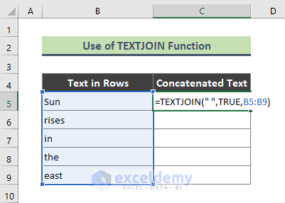
- Hit Enter.
Method 6 – Joining TRANSPOSE and CONCATENATE Functions to Add Rows
Combine the TRANSPOSE function along with the CONCATENATE function to get a joined text from selected rows.
Steps:
- Type the below formula in Cell C5 but do not press Enter.
=TRANSPOSE(B5:B7)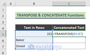
- Put the cursor on the above formula and press F9 from the keyboard. The formula will look like the below image. Remove both of the curly brackets from the formula.
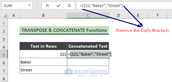
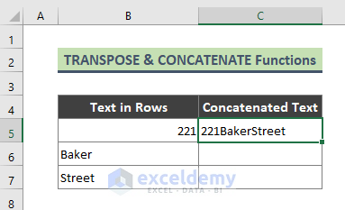
- After deleting the curly brackets, type CONCATENATE before the first value and close the formula with parentheses. The formula looks like below:
=CONCATENATE(221,"Baker","Street")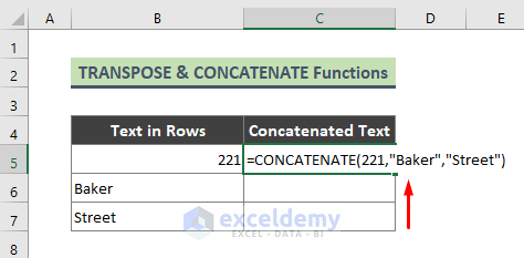
- Press Enter.
Related Content: Opposite of Concatenate in Excel (4 Options)
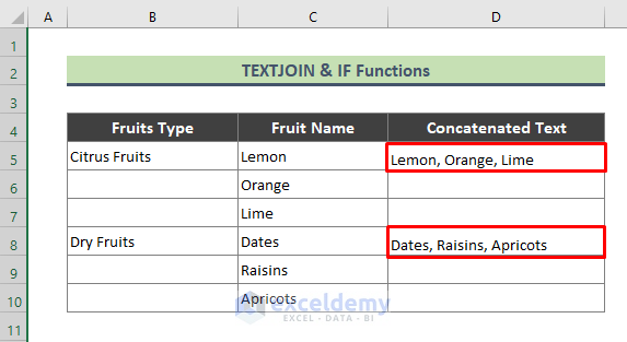
Method 7 – Merging Excel IF and TEXTJOIN Functions to Concatenate Multiple Rows
Use IF and TEXTJOIN functions to combine strings from rows.
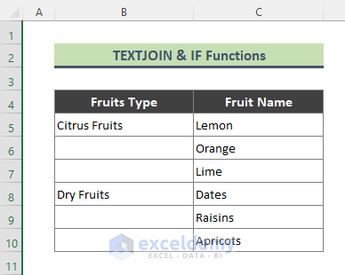
In the sample dataset (B5:C10) contains fruit types in column B and fruit names in column C.
We can combine all the fruit names in a fruit type category and concatenate the result.
Steps:
- Type the below formula in Cell D5 and press Enter.
=IF(B5="","",TEXTJOIN(", ",TRUE,C5:C7))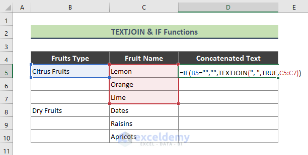
- Use the Fill Handle to copy the formula to the rest of the cells.
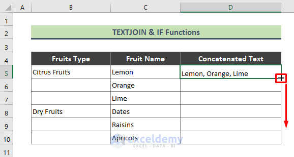
- All the fruits under a certain category are concatenated as below.
Related Content: How to Concatenate Multiple Cells in Excel (8 Quick Approaches)
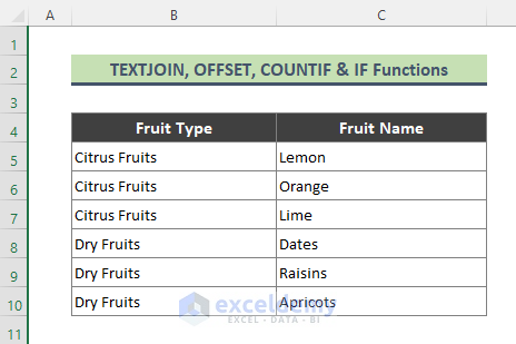
Method 8 – Combining TEXTJOIN, OFFSET, and COUNTIF Functions to Add Rows
Combine TEXTJOIN, OFFSET, COUNTIF, and IF functions to join rows in Excel.
The sample dataset contains fruit types and fruit names. We can merge the fruits according to their type.
Steps:
- Type the below formula in Cell D5 and press Enter.
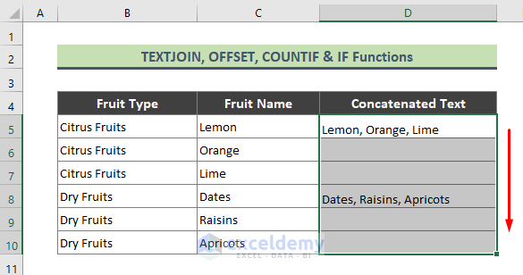
=IF(B5=B4,"",TEXTJOIN(", ",TRUE,OFFSET(C5,0,0,COUNTIF(B:B,B5),1)))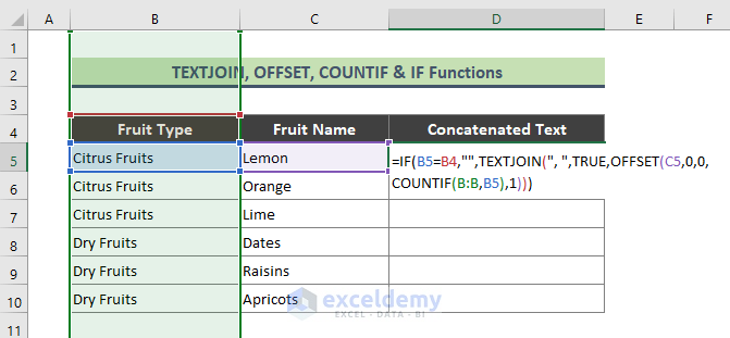
- Use the Fill Handle to copy the formula to the rest of the cells.
How Does the Formula Work?
➤ COUNTIF(B:B,B5)
This part of the formula returns:
{3}
➤ OFFSET(C5,0,0,COUNTIF(B:B,B5),1)
This part returns:
{$C$5:$C$7}
➤ TEXTJOIN(“, “,TRUE,C$5:$C$7)
This part returns:
{Lemon,Orange,Lime}
➤ IF(B5=B4,””,TEXTJOIN(“, “,TRUE,OFFSET(C5,0,0,COUNTIF(B:B,B5),1)))
Applying the B5=B4 condition returns:
{Lemon,Orange,Lime}
Method 9 – Using Fill Justify Command to Join Rows in Excel
Steps:
- Select the range (B5:C9).
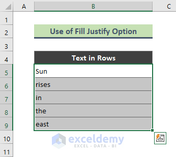
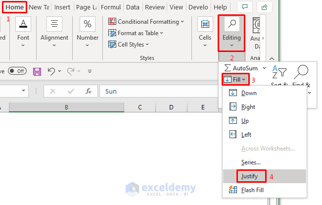
- Go to Home > Editing > Fill > Justify.
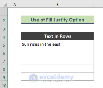
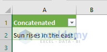
- All the text from the selected rows will be joined.
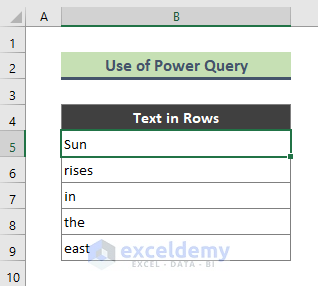
Method 10 – Using Excel Power Query Tool to Add Rows
Steps:
- Select anywhere on the dataset.
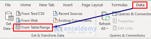
- Go to Data > From Table/Range option.
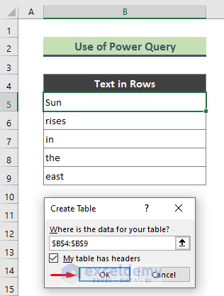
- The Create Table dialog will appear, check the table range, and click OK.
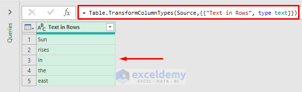
- A table will be visible in the Power Query Editor window.
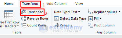
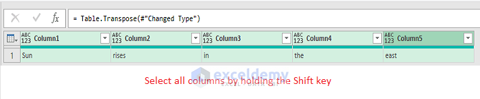
- From the Power Query Editor, go to Transform > Transpose.
- The text will be separated into several columns. Select all the columns by pressing the Shift + ➝ keys.
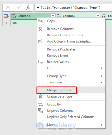
- Right-click on the selection and click on Merge Columns.
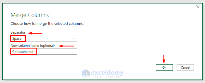
- The Merge Columns dialog will appear. Choose ‘Space’ as the Separator, type the New column name, and click OK.
- The text will be concatenated in a single cell.
- Go to Home > Close & Load > Close & Load to close the Power Query Editor.
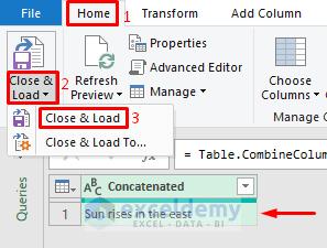
- The result is now concatenated in the spreadsheet.
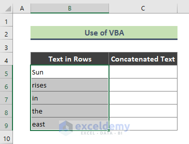
Method 11 – Concatenating Rows in Excel Using VBA Macro
Steps:
- Select the range (B5:B9).
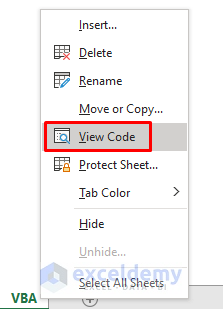
- Right-click on the sheet name and click on the View Code to bring the VBA window. Yow can also use Alt + F11 too keys to bring the VBA window.
- Enter the below code in the Module and run by pressing the F5 key. Specify in the Range where you want to see the concatenated text. I have put C5 as I want to see my result in Cell C5.
 Sub ConcatenateText()

 Dim text As Range
 Dim i As String
 For Each text In Selection
 i = i & text & " "
 Next text
 Range("C5").Value = Trim(I)

 End Sub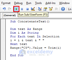
Things to Remember
➨ You can use both the CONCATENATE function and Ampersand (&) operator to join rows in excel. However, the CONCATENATE function can only join up to 255 strings.
➨ You cannot pass a range through the CONCATENATE function. Each of the cells must be referenced separately as: =CONCATENATE(B5,” “,B6,” “,B7,” “,B8,” “,B9).
Download Practice Workbook
You can download the practice workbook that we have used to prepare this article.
<< Go Back to Range | Concatenate | Learn Excel
Get FREE Advanced Excel Exercises with Solutions!
