Method 1 – Selecting Label Contains Option
Step 1:
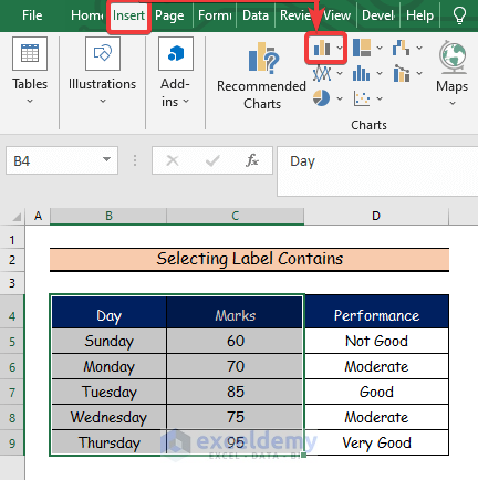
- Select the B and C columns.
- Select the Insert tab.
- Select the Insert Column or Bar Chart.
Step 2:
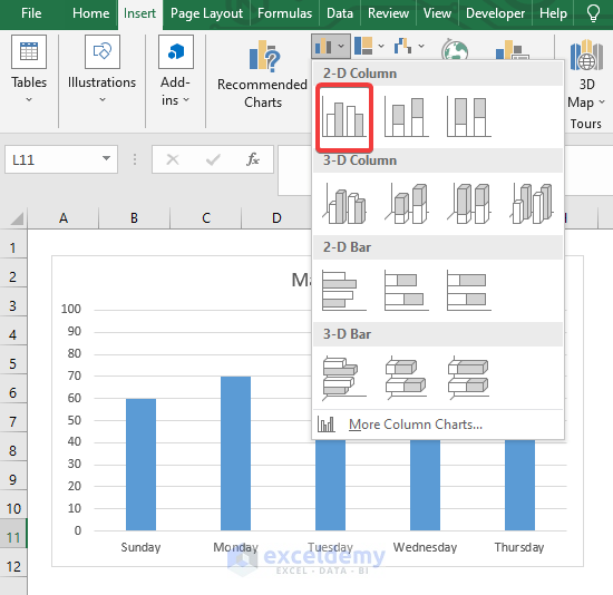
- Click the 2D Column chart option.
Step 3:
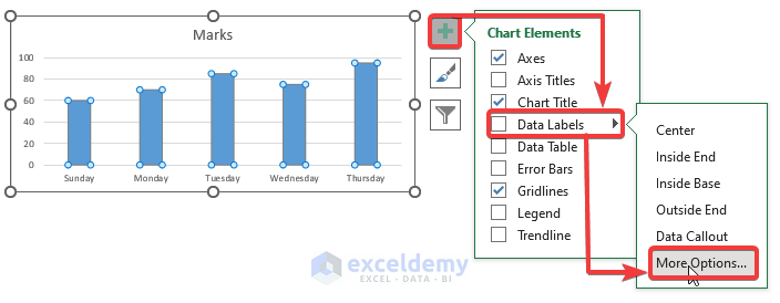
- Go to the Data Labels command from the Chart Element option.
- Click on More Options.
Step 4:
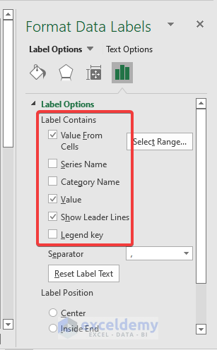
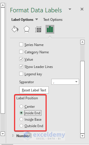
- The Format Data Labels panel will open.
- Select any option you want from the Label Options.
- Choose three options, including Value From Cells, Value, and Show Leader Lines.
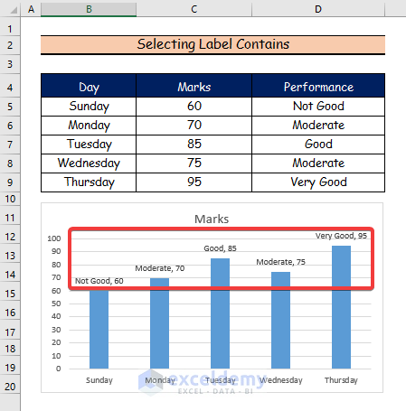
Step 5:
- When you use the Label Contains options to update the data labels, the results are as follows.
Method 2 – Altering Label Positions to Edit Data Labels
Step 1:
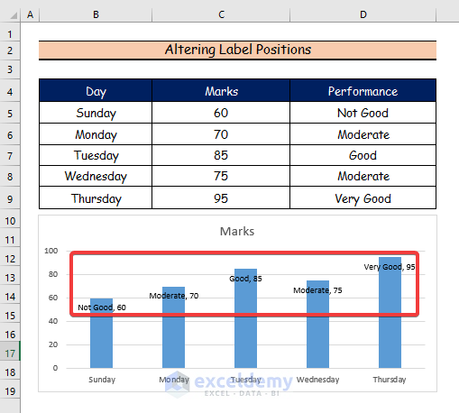
- Select one of the options from the Label Position Click on the Inside End option.
Step 2:
- Observe the following outcomes when using the Label Position command to edit data labels.
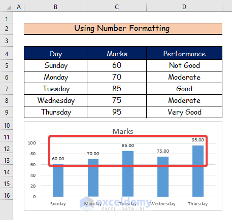
Method 3 – Formatting Number to Edit Data Labels
Step 1:
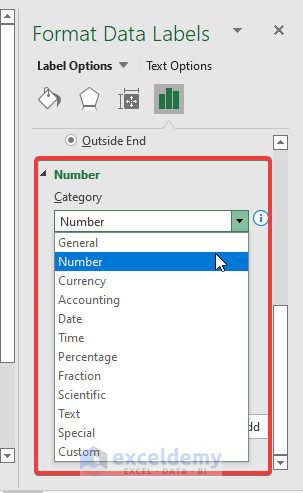
- Select a Number Format choice from each list. In this case, we will select the Number option.
Step 2:
- The results of modifying data labels with two decimal places will be as follows.
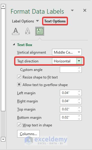
Method 4 – Changing Text Directions
Step 1:
- Pick a Text Directions option from the list. Use the Horizontal Text Direction option.
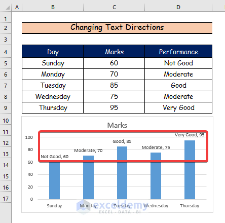
Step 2:
- The final set of outcomes for editing data labels with horizontal text direction is shown below.
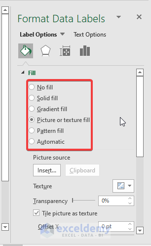
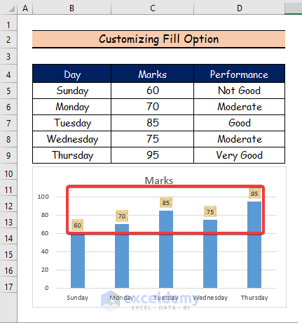
Method 5 – Customizing Fill Option to Edit Data Labels
Step 1:
- The Fill menu now. We will select the Picture or texture fill command in this case.
Step 2:
- You will see the following outcomes when using the Picture Fill or Texture Fill commands to alter data labels.
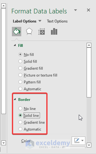
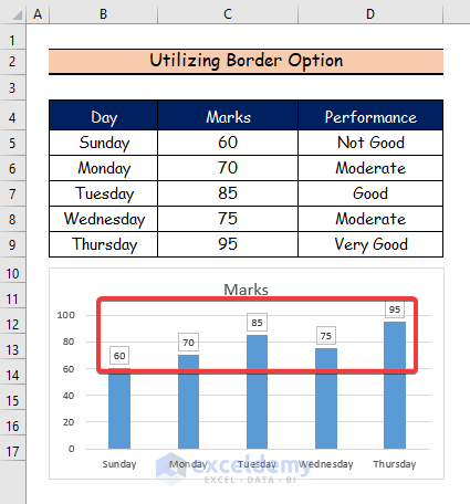
Method 6 – Utilizing Border Option to Edit Data Labels
Step 1:
- Choose a command from the Border choice by doing so. We will choose the Solid line option in this instance.
Step 2:
- The following results for altering data labels with a Solid line border are the last ones you will see.
You may download the following Excel workbook for better understanding and practice yourself.
Related Articles
- How to Remove Zero Data Labels in Excel Graph
- How to Hide Zero Data Labels in Excel Chart
- [Fixed:] Excel Chart Is Not Showing All Data Labels
- How to Change Font Size of Data Labels in Excel
<< Go Back To Data Labels in Excel | Excel Chart Elements | Excel Charts | Learn Excel

