How to Remove Zero Data Labels in Excel Graph (3 Easy Ways)

If you are looking for ways to remove zero data labels in an Excel graph, this article is for you. So, let’s start with the main article to know detailed procedures for removing zero data labels.

How to Remove Zero Data Labels in Excel Graph: 3 Ways

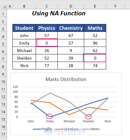
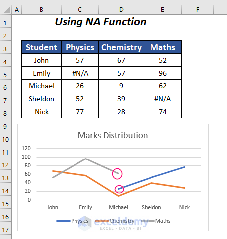
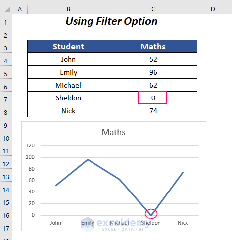
Here, we have the following dataset containing records of marks for 3 subjects of some students. Among the students, two of them got 0 in two different subjects. After plotting them as Line Chart, Column Chart, and Pie Chart we can see that the Line Chart is conspicuously showing zero data labels. Seemingly, the other two forms are avoiding the zero data labels. So, in the following sections, we will discuss more of the ways to remove the zero data labels from the Line Chart.

We have used Microsoft Excel 365 version for this article, you can use any other version according to your convenience.

Method-1: Using NA Function to Remove Zero Data Labels in Excel Graph

In this method, we are going to replace zero in Physics for Emily and in Maths for Sheldon with #N/A to avoid zero data labels.

Read More: What Are Data Labels in Excel

Case-01: Usage of NA Function with Find and Replace Option

Here, we will replace the normal zero values with #N/A using the NA function.

Steps:
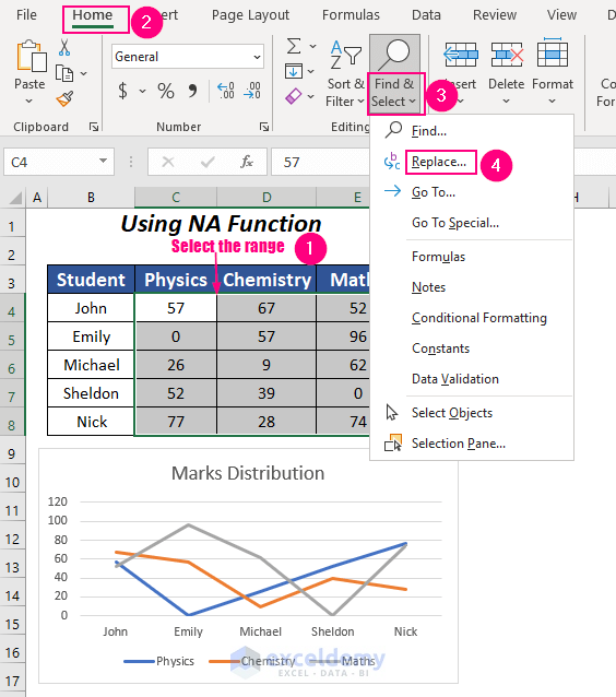
Firstly, we have to find the zero values in the dataset and then replace them with #N/A.
➤ Select the range and then go to the Home Tab >> Editing Group >> Find & Select Dropdown >> Replace Option.

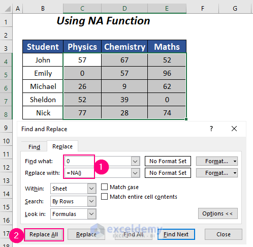
After that, the Find and Replace dialog box will open up.
➤ Type the following in the first two boxes.
Find what → 0
Replace with → =NA()
➤ Select the Replace All option.

Afterward, the Microsoft Excel message box will appear which informs about 2 replacements.
➤ Click on OK.

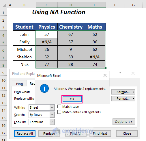
After that, the zero values will be replaced by #N/A and the graphs are not showing zero data labels here anymore.

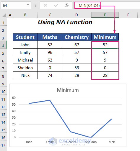
Case-02: Usage of NA Function for Formula

Here, we will show the way of replacing zero with #N/A in a formula. In the Minimum column, we have used the MIN function to have the minimum value between the marks of Maths and Chemistry and the graph is showing the minimum values with zero data label.

Steps:
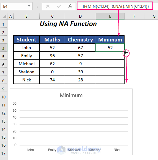
➤ After removing the previous formula, enter the following formula in cell E4.

=IF(MIN(C4:D4)=0,NA(),MIN(C4:D4))

If the minimum value is zero then the IF function will return #N/A otherwise the minimum value.

➤ Drag down the Fill Handle tool.

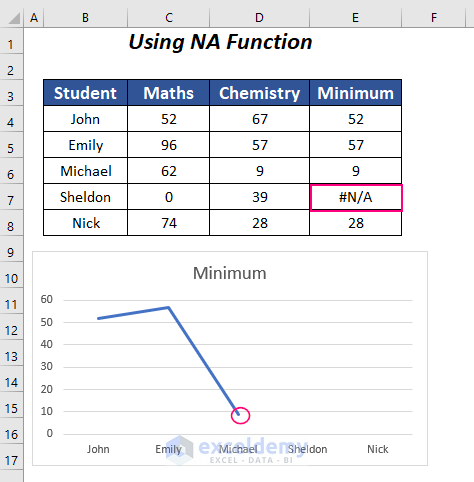
In this way, the Zero value for Sheldon has been superseded with #N/A. And the graph has also removed zero data labels.

READ MORE: How to Add Data Labels in Excel

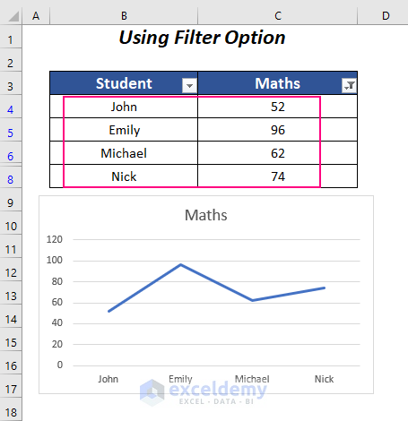
Method-2: Using Filter Option to Remove Zero Data Labels in Excel Graph

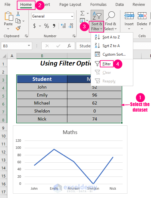
This method can only be used if your graph is plotted with single column values like we have plotted the following graph for the students with their Maths number only.

Steps:
➤ Select the dataset and then go to the Home Tab >> Editing Group >> Sort & Filter Dropdown >> Filter Option.

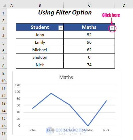
Then, the filter dropdown option will appear on the column headers.
➤ Click on the dropdown symbol in the Maths column.

➤ Uncheck the box with the number 0 and then press OK.

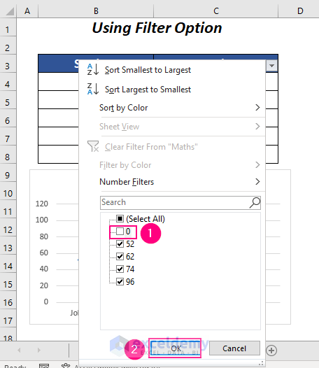
Finally, we have removed the marks 0 in the row for Sheldon and our graph has also eliminated this 0 data label.

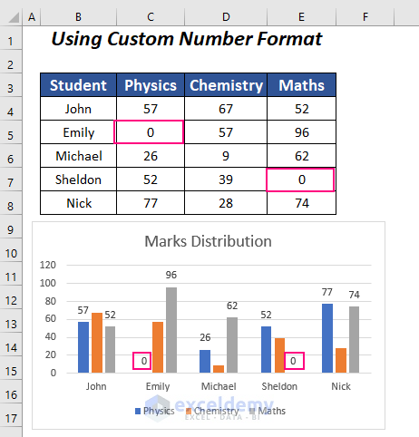
Method-3: Using Custom Number Format to Format Data Labels of Chart

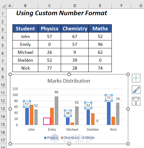
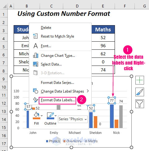
Without data labels, column charts may ignore zero data labels, but when we activate the data label option of the chart we can see the zero data labels for the Physics and Maths series also in the chart. To remove this label you can follow this section.

Steps:
➤ Select the data labels of the Physics series and then Right-click here.
➤ Choose the Format Data Labels option.

On the right side, the Format Data Labels wizard will appear.
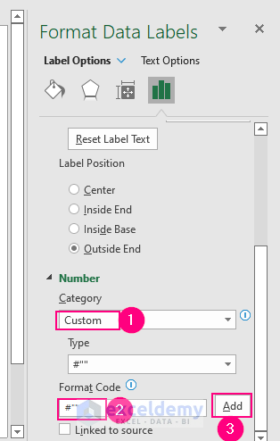
➤ Go to the Label Options and then scroll down to the following options.

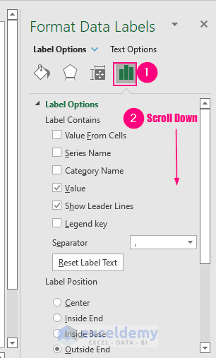
➤ Under the Number option, select the Category as Custom, in the Format Code box type #”” and click on the Add button.

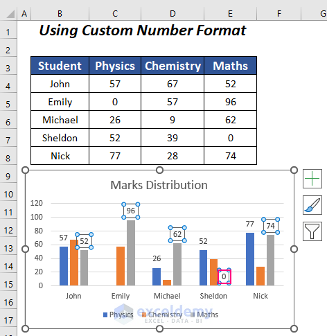
In this way, we have removed the zero data label from the Physics series.

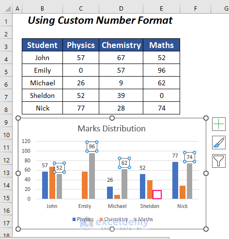
Similarly, we will remove the zero data label from the selected Maths series as well.

Finally, we have removed all of the zero data labels from the following chart.

Read More: How to Format Data Labels in Excel

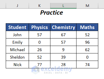
Practice Section

For doing practice by yourself we have provided a practice section like below in each sheet on the right side. Please do it by yourself.

Download Workbook

Remove Zero Data Labels.xlsx

Conclusion

In this article, we tried to remove zero data labels in an Excel graph. Hope you will find it useful. If you have any suggestions or questions, feel free to share them in the comment section.

<< Go Back To Data Labels in Excel | Excel Chart Elements | Excel Charts | Learn Excel

Get FREE Advanced Excel Exercises with Solutions!