While working in Microsoft Excel you might need to show your data in different directions for better visualization. You can change the direction of your data labels in various positions. In this article, I am going to share with you how to rotate data labels in Excel.
How to Rotate Data Labels in Excel: 2 Easy Methods
In the following article, I am describing 2 easy and simple methods to rotate data labels in Excel.
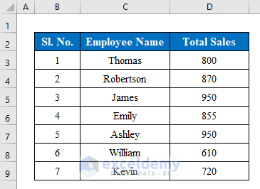
Suppose we have a dataset of some Employee Names and their Total Sales.
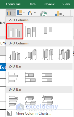
Firstly, we will create a 2-D chart. To do so select data from the table and go to the “Insert” option.

From the chart, options choose a 2-D chart of your choice.
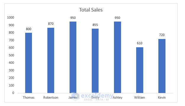
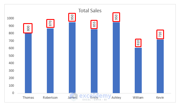
Finally, you will get a 2-D chart ready to display your chosen data. Now we will rotate the data labels inside the bar chart by applying some suitable methods.
Read More: How to Add Data Labels in Excel
1. Use Format Data Labels Option to Rotate Data Labels
The simplest way to rotate data labels is by using format data labels. Check the following steps below-
Steps:
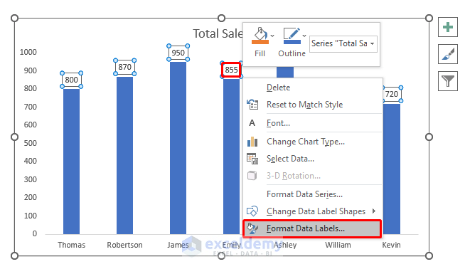
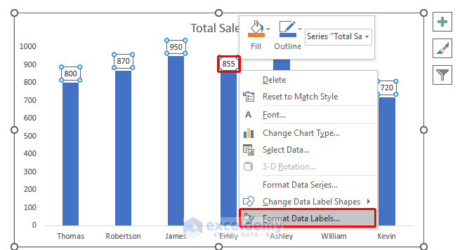
- Select any data labels from the inserted chart. Here I have selected the sales volume of each employee.
- Right-click the mouse button to appear options. From the options click “Format Data Labels”.
- A right pane will appear on the right side of the workbook.
- From the “Format Data Labels” pane firstly click the “Text Options”.
- After that choose “Text Box” and from the drop-down list of “Text direction” press the “Rotate all text 270°”.
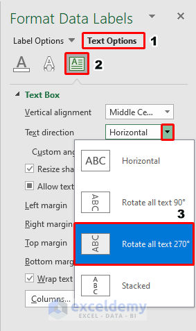
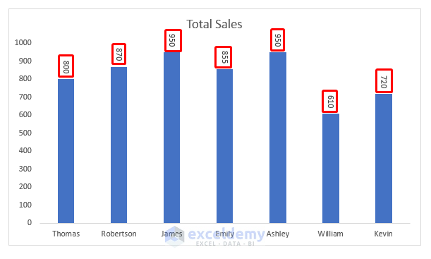
- Here we have our data labels rotated in a vertical way just by changing the text direction.
Read More: How to Format Data Labels in Excel
2. Utilize Format Axis Feature to Rotate Data Labels
You can also utilize the format axis if you want to rotate the data labels. Follow the steps below to learn the process-
Steps:
- Choosing data labels right-click the mouse button to get options.
- Click “Format Data Labels”.
- From the “Format Data Labels” pane press the “Size and Properties” icon.
- Now, in the alignment section change the text direction to “Rotate all text to 90°”.

- As you can see we have our desired result ready rotating the data labels to 90°.
Read More: How to Move Data Labels In Excel Chart
Things to Remember
- In this article, I have changed the direction of numbers. If you want you can change the text direction too following the same processes described above.
Download Practice Workbook
Download this practice workbook to exercise while you are reading this article.
Conclusion
In this article, I have tried to cover all the simple steps to rotate data labels in Excel. Take a tour of the practice workbook and download the file to practice by yourself. Hope you find it useful. Please inform us in the comment section about your experience.
Related Articles
- How to Edit Data Labels in Excel
- How to Change Font Size of Data Labels in Excel
- How to Remove Zero Data Labels in Excel Graph
- How to Hide Zero Data Labels in Excel Chart
- [Fixed:] Excel Chart Is Not Showing All Data Labels
<< Go Back To Data Labels in Excel | Excel Chart Elements | Excel Charts | Learn Excel
Get FREE Advanced Excel Exercises with Solutions!
