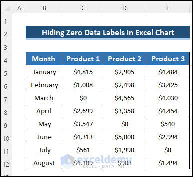
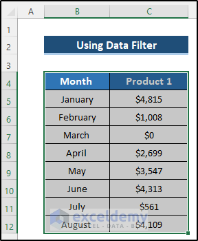
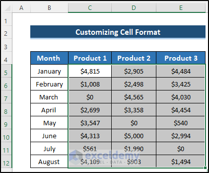
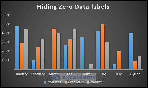
How to Hide Zero Data Labels in an Excel Chart

The dataset showcases months and sales amounts of different products .

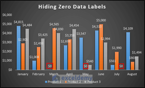
When you plot that dataset in an Excel chart, zero data labels are displayed.

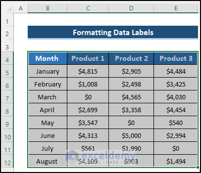
Method 1 – Formatting the Data Labels

The dataset contains several zeros.

Steps

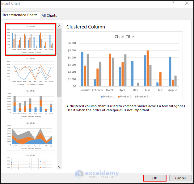
Select B4:E12.

Go to the Insert tab.
In Charts, select Recommended Charts.

In the Insert Chart dialog box, select Clustered Column.
Click OK.

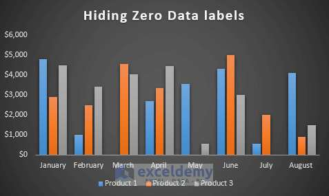
After changing the chart style, this is the output.

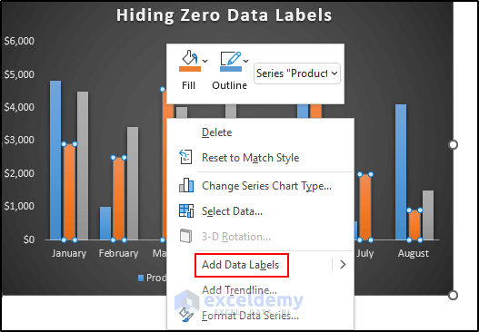
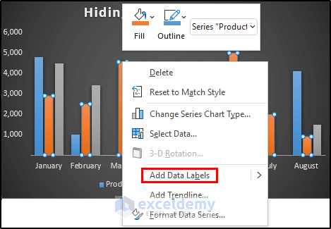
Right-click the column to open the Context Menu.
Select Add Data Labels.

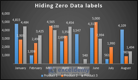
This is the output.

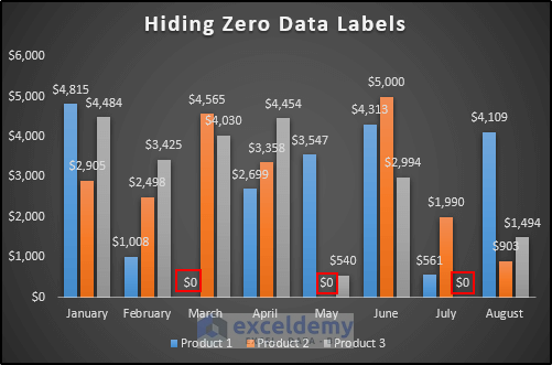
As zero values represent three product values, you need to modify each one of them.
Right-click any zero value, and select Format Data Labels.

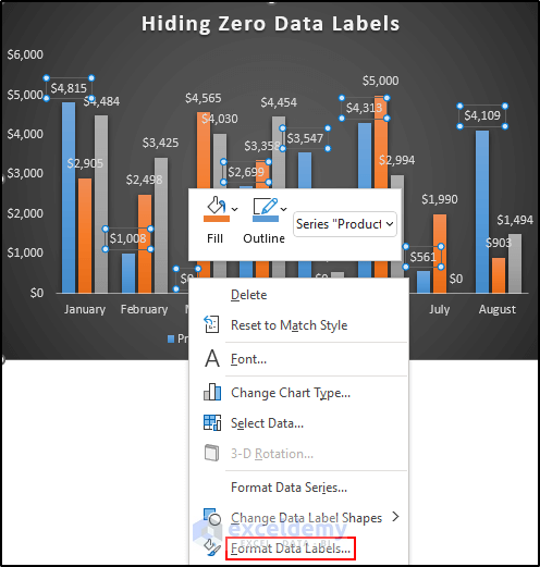
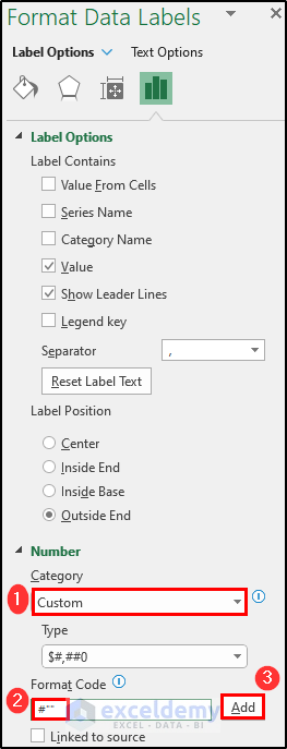
In the Format data labels dialog box, select Label Options and choose Number.
In Category, select Custom.
In Format Code, enter the following

#””

Click Add.

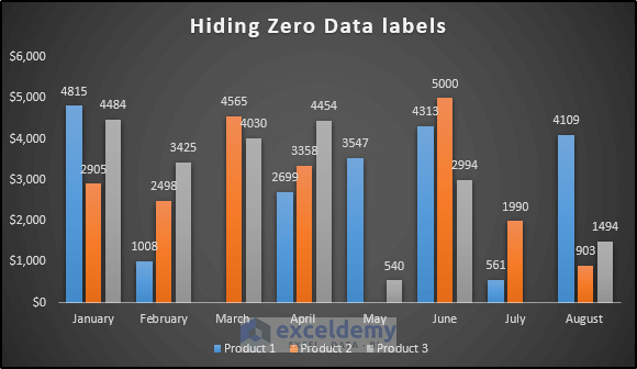
The zero data label is hidden.

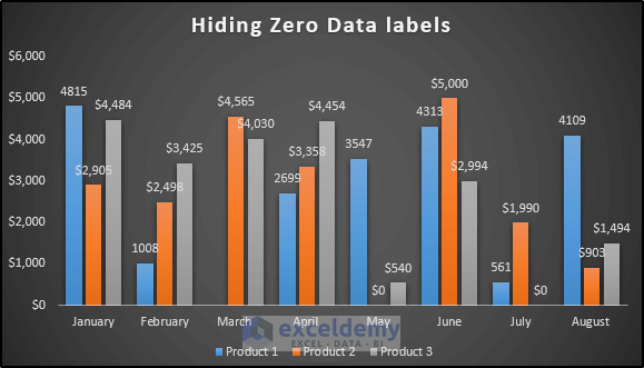
To hide the other two zero data labels, follow the same procedure. This is the ouput.

Read More: How to Edit Data Labels in Excel

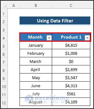
Method 2 – Using the Data Filter

Steps

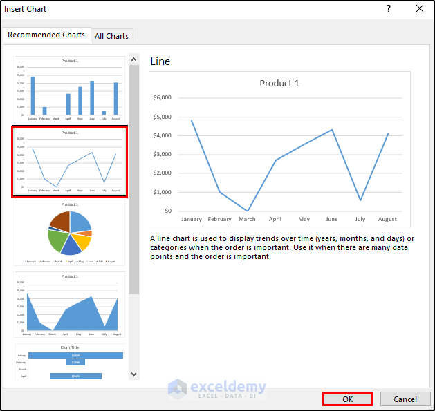
Select B4:C12.

Go to the Insert tab.
In Charts, select Recommended Charts.

In the Insert Chart dialog box, select Line.
Click OK.

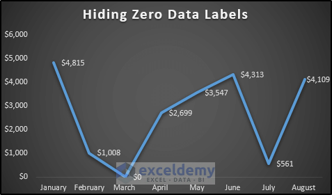
This is the output.

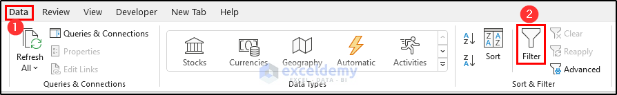
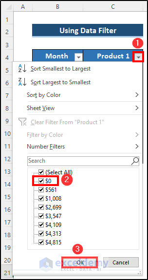
To filter the dataset and hide zero data labels, select B4:C12.
Go to the Data tab.
Select Filter in Sort & Filter.

You will see the filter drop-down option.

Click the filter drop-down.
Uncheck zero (0).
Click OK.

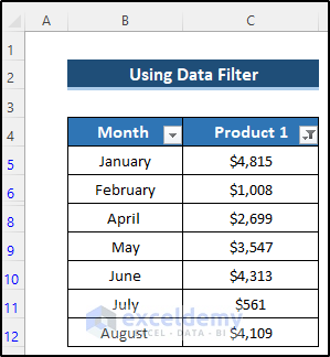
This is the output.

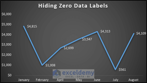
This is the Excel chart.

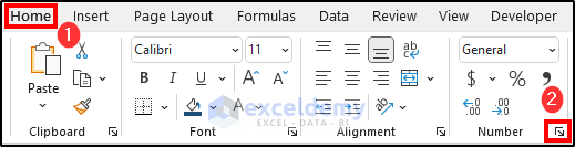
Method 3 – Customizing the Cell Format

Steps

Select C5:E12.

Go to the Home tab.
Select Format Cells Dialog launcher in Number.

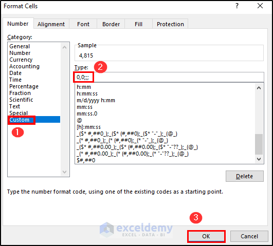
In the Format Cells dialog box, select Custom in Category.
Enter the following in Type.

0,0;;;

Click OK.

All zero values are hidden.

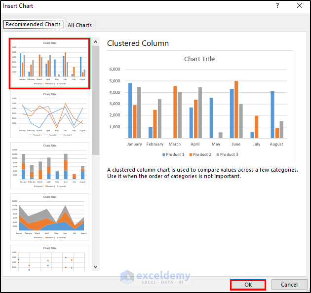
To plot that dataset in an Excel chart, select B4:E12.

Go to the Insert tab and in Charts, select Recommended Charts.

In the Insert Chart dialog box, select Clustered Column.
Click OK.

After changing the chart style, this is the output.

If you add data labels, you won’t see zeros.
Right-click the column to open the Context Menu.
Select Add Data Labels.

This is the output.

Method 4 – Applying the NA Function

Steps

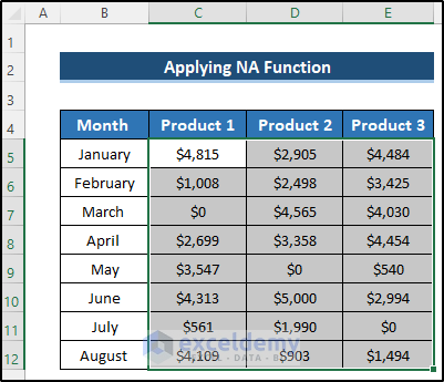
Replace the zero values with the NA function.
Select C5:E12.

Go to the Home tab.
In Editing, select Find & Select.

Select Replace in Find & Select.

In the Find and Replace dialog box, set Find what as 0.
Enter the following formula in Replace with.

=NA()

Select Find Next.
Click Replace.
As there are several zero values, you need to find and replace them one by one and replace.

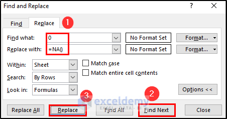
Click Close.
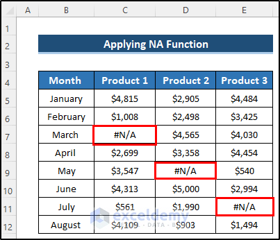
This is the output.

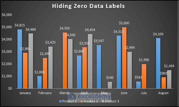
This is the Excel chart.

Things to Remember

While using the NA function in Find & Select, you may face problems if you apply Replace All because there are zeros in non-zero numbers like $4030. Excel can’t differentiate them and will replace them also.

Download Practice Workbook

Download the practice workbook below.

Hide Zero Data labels in Excel Chart.xlsx

<< Go Back To Data Labels in Excel | Excel Chart Elements | Excel Charts | Learn Excel

Get FREE Advanced Excel Exercises with Solutions!

How to Hide Zero Data Labels in an Excel Chart – 4 Methods

Method 1 – Formatting the Data Labels

Method 2 – Using the Data Filter

Method 3 – Customizing the Cell Format

Method 4 – Applying the NA Function

Things to Remember

Related Articles

Leave a reply Cancel reply