How to Change Font Size of Data Labels in Excel

This tutorial will demonstrate how to change the font size of data labels in Excel charts using 2 different examples.

Example 1 – Changing the Font Size of Data Labels for a 2-D Column Chart

The point of changing the font size of data labels in Excel is to make the graph or data more visually attractive and understandable. Let’s change the font size of the labels on a 2-D Column chart:

Steps:

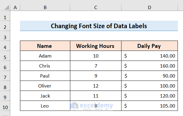
Suppose we have a dataset of people with their Working Hours in Column C and Daily Pay in Column D.

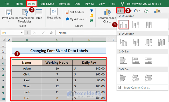
Select the whole dataset and go to the Insert tab.
Click on the Insert Pie or Doughnut Chart icon and select 2-D Column.

Select the whole graph, click on the Chart Elements option and go to the Data Labels.

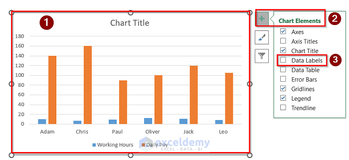
The result will be like the image below.

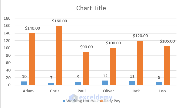
Select a label on the chart and go to the Home tab.
Choose an appropriate font size.

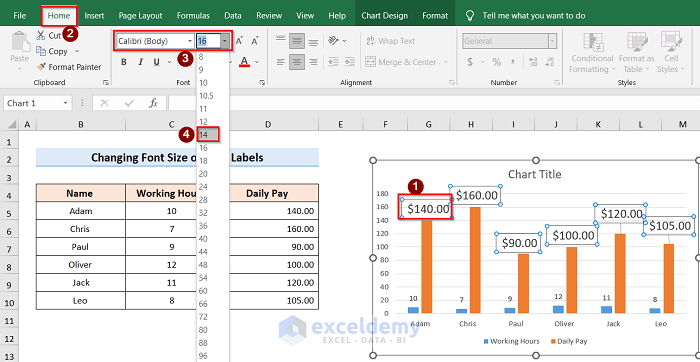
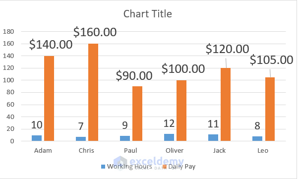
The following is the result:

Read More: How to Edit Data Labels in Excel

Example 2 – Modifying the Font Size of the Data Labels for a Pie Chart

Using the same dataset as the first example, let’s now modify the font size of the data labels for a Pie Chart.

Steps:

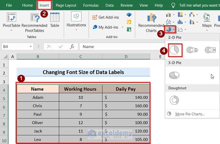
Select the whole dataset and go to the Insert tab.
Click on the 2-D Pie icon.

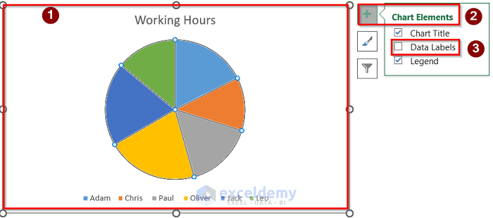
After generating a pie chart, select the whole chart and choose Data Labels from the Chart Elements.

Select the chart and go to the Home tab.
Choose an appropriate font size.

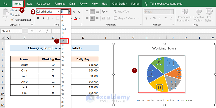
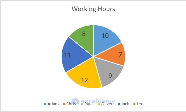
The following is the result:

Read More: How to Format Data Labels in Excel

Things to Remember

It is recommended to never use the 3-D Pie or 3-D Column Chart options because they’re confusing and open to misinterpretation.
Change the font such that the text becomes easily understandable. It is recommended to keep enough space between the labels so that the chart doesn’t become cluttered and difficult to interpret.

Download Practice Workbook

Change Font Size of Data Labels.xlsx