#VALUE! error is a common error in Excel. This error occurs when there is something wrong with the way you typed the formula or the cells you are referring to in the formula. You can face this error while using different functions in Excel. The main objective of this article is to explain the reasons behind the AVERAGEIFS Value (#VALUE!) error in Excel and how you can fix it.
How to Fix AVERAGEIFS Value (#VALUE!) Error in Excel: 3 Reasons with Solutions
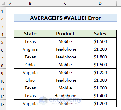
Here, I have taken the following dataset to explain this article. This dataset contains the State, Product, and Sales. I will explain 3 different reasons and solutions for the AVERAGEIFS Value (#VALUE!) error in Excel.
1. Selecting Wrong Criteria Range in Excel
The first reason behind the AVERAGEIFS Value (#VALUE!) error is selecting the wrong criteria range in the formula.
In the following image, you can see that the cell range B5:C13 is selected as criteria_range1 and C16 as criteria1. While criteria1 is in the cell range B5:B13. The same thing happened for ctiteria_range2. The criteria2 is in cell range C5:C13 but B5:C13 is selected as criteria_range2 in the formula. For this reason, the formula is showing a #VALUE! error.

Now, I will show you how you can fix this error.
Solution: Selecting the Right Criteria Range
You can easily solve this error by selecting the criteria_range carefully in the AVERAGEIFS function.
- Firstly, select the cell where you want to fix the AVERAGEIFS Value error. Here, I selected cell C19.
- Secondly, in cell C19 write the following formula.
=AVERAGEIFS(D5:D13,B5:B13,C16,C5:C13,C17)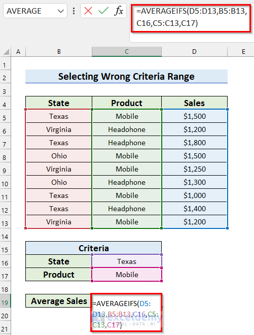
- Thirdly, press Enter and you will get your desired result.
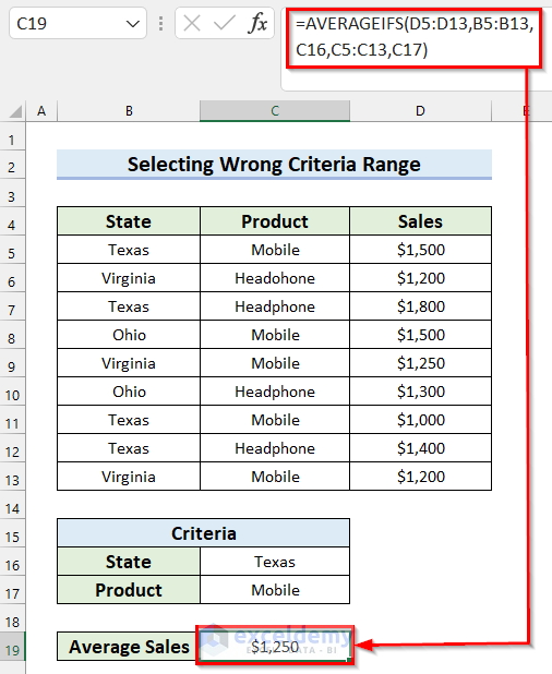
Here, in the AVERAGEIFS function, I selected cell range D5:D13 as average_range, cell rage B5:B13 as criteria_range1, C16 as criteria1, cell range C5:C13 as criteria_range2, and C17 as criteria2.
Read More: Excel AVERAGEIFS with Multiple Criteria in Same Range
2. Using Different Types of Cell Ranges at Same Time
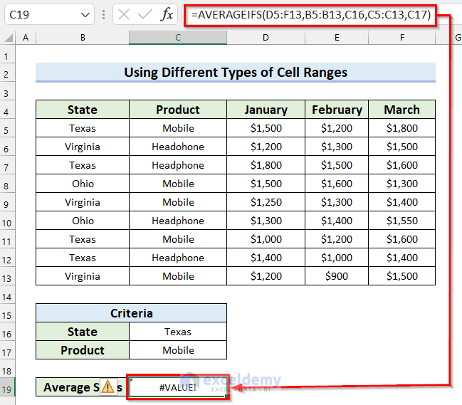
The second reason behind the AVERAGEIFS Value (#VALUE!) error is using different types of cell ranges at the same time.
In the following image, you can see that the dataset contains Sales for 3 Months. Suppose I want to calculate Average Sales for Mobile in Texas. Now, you can see that in the AVERAGEIFS function, cell range D5:F13 is selected as average_range. This cell range contains multiple columns. Here, cell range B5:B13 is selected as criteria_range1, and cell range C5:C13 is selected as criteria_range2. Both of these ranges contain only one column. But you can not select both single column range and multiple columns range in the AVERAGEIFS function at the same time and for this reason, the formula is showing #VALUE! error.
Let’s see how you can fix this error.
Solution: Using AVERAGE and IF Functions
You can fix this error by using the AVERAGE function and the IF function instead of the AVERAGEIFS function and get your desired result.
- Firstly, select the cell where you want to calculate the Average Sales.
- Secondly, write the following formula in the selected cell.
=AVERAGE(IF(B5:B13=C16,IF(C5:C13=C17,D5:F13)))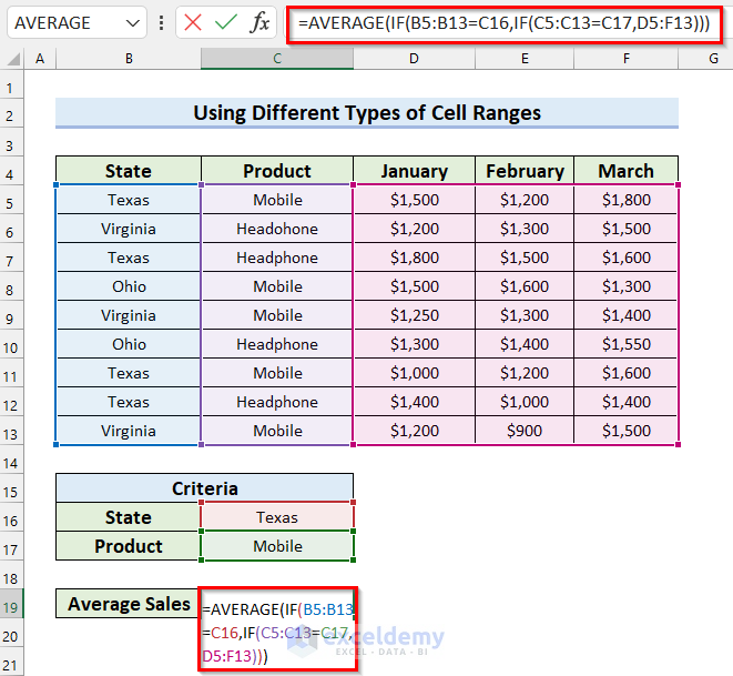
- Finally, press Enter to get the result. But, if you are using an older version of Microsoft Excel than Excel 2019 then press Ctrl + Shift + Enter to get the result.

🔎 How Does the Formula Work?
- IF(C5:C13=C17,D5:F13) —-> Here, the IF function will check if the value in cell C17 matches the values in cell range C5:C13. If the logical_test is True then it will return cell range D5:F13 otherwise it will return FALSE.
- Output: {1500,1200,1800;FALSE,FALSE,FALSE;FALSE,FALSE,FALSE;1500,1600,1300;1250,1300,1400;FALSE,FALSE,FALSE;1000,1200,1600;FALSE,FALSE,FALSE;1200,900,1500}
- IF(B5:B13=C16,IF(C5:C13=C17,D5:F13)) —-> turns into
- IF(B5:B13=C16,{1500,1200,1800;FALSE,FALSE,FALSE;FALSE,FALSE,FALSE;1500,1600,1300;1250,1300,1400;FALSE,FALSE,FALSE;1000,1200,1600;FALSE,FALSE,FALSE;1200,900,1500}) —-> Now, the IF function will check if the value in cell C16 matches the values in cell range B5:B13. If the logical_test is True then it will return values from the array otherwise it will return FALSE.
- Output: {1500,1200,1800;FALSE,FALSE,FALSE;FALSE,FALSE,FALSE;FALSE,FALSE,FALSE;FALSE,FALSE,FALSE;FALSE,FALSE,FALSE;1000,1200,1600;FALSE,FALSE,FALSE;FALSE,FALSE,FALSE}
- IF(B5:B13=C16,{1500,1200,1800;FALSE,FALSE,FALSE;FALSE,FALSE,FALSE;1500,1600,1300;1250,1300,1400;FALSE,FALSE,FALSE;1000,1200,1600;FALSE,FALSE,FALSE;1200,900,1500}) —-> Now, the IF function will check if the value in cell C16 matches the values in cell range B5:B13. If the logical_test is True then it will return values from the array otherwise it will return FALSE.
- AVERAGE(IF(B5:B13=C16,IF(C5:C13=C17,D5:F13))) —-> turns into
- AVERAGE({1500,1200,1800;FALSE,FALSE,FALSE;FALSE,FALSE,FALSE;FALSE,FALSE,FALSE;FALSE,FALSE,FALSE;FALSE,FALSE,FALSE;1000,1200,1600;FALSE,FALSE,FALSE;FALSE,FALSE,FALSE}) —-> Here, the AVERAGE function will calculate the average of the values.
- Output: 1383
- AVERAGE({1500,1200,1800;FALSE,FALSE,FALSE;FALSE,FALSE,FALSE;FALSE,FALSE,FALSE;FALSE,FALSE,FALSE;FALSE,FALSE,FALSE;1000,1200,1600;FALSE,FALSE,FALSE;FALSE,FALSE,FALSE}) —-> Here, the AVERAGE function will calculate the average of the values.
Read More: How to Use AVERAGEIFS Function for Multiple Columns
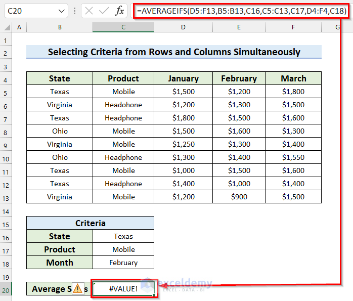
3. Selecting Criteria from Rows and Columns Simultaneously
The third reason behind AVERAGEIFS Value (#VALUE!) error is selecting criteria from rows and columns simultaneously. The AVERAGEIFS function can not work with this kind of data as a result it returns #VALUE! error.
In the following image, you can see that cell range B5:B13 is selected as criteria_range1, C5:C13 is selected as criteria_range2, and D4:F4 is selected as criteria_range3. Here, criteria_range1 and criteria_range2 are columns but criteria_range3 is a row. And for this reason, the formula is showing a #VALUE! error.
Let me show you how you can fix this AVERAGEIFS Value error in Excel.
Solution: Employing Array Formula
You can easily solve this problem by using an array formula.
- Firstly, select the cell where you want to fix this error. Here, I selected cell C20.
- Secondly, in cell C20 write the following formula.
=AVERAGE(IF(B5:B13=C16,IF(C5:C13=C17,IF(D4:F4=C18,D5:F13))))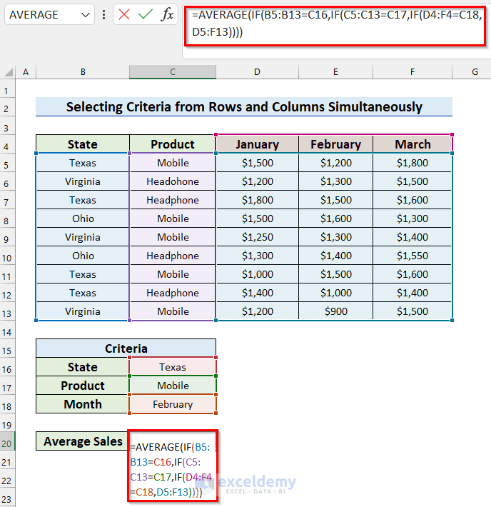
- After that, press Enter to get the result. If you are using an older version of Microsoft Excel than Excel 2019 then press Ctrl + Shift + Enter to get the result.

🔎 How Does the Formula Work?
- IF(D4:F4=C18,D5:F13) —-> Here, the IF function will check if the value in cell C18 matches the values in cell range D4:F4. If the logical_test is True then it will return cell range D5:F13 otherwise it will return FALSE.
- Output: {FALSE,1200,FALSE;FALSE,1300,FALSE;FALSE,1500,FALSE;FALSE,1600,FALSE;FALSE,1300,FALSE;FALSE,1400,FALSE;FALSE,1500,FALSE;FALSE,1000,FALSE;FALSE,900,FALSE}
- IF(C5:C13=C17,IF(D4:F4=C18,D5:F13)) —-> turns into
- IF(C5:C13=C17,{FALSE,1200,FALSE;FALSE,1300,FALSE;FALSE,1500,FALSE;FALSE,1600,FALSE;FALSE,1300,FALSE;FALSE,1400,FALSE;FALSE,1500,FALSE;FALSE,1000,FALSE;FALSE,900,FALSE}) —-> Now, the IF function will check if the value in cell C17 matches the values in cell range C5:C13. If the logical_test is True then it will return values from the array otherwise it will return FALSE.
- Output: {FALSE,1200,FALSE;FALSE,FALSE,FALSE;FALSE,FALSE,FALSE;FALSE,1600,FALSE;FALSE,1300,FALSE;FALSE,FALSE,FALSE;FALSE,1500,FALSE;FALSE,FALSE,FALSE;FALSE,900,FALSE}
- IF(C5:C13=C17,{FALSE,1200,FALSE;FALSE,1300,FALSE;FALSE,1500,FALSE;FALSE,1600,FALSE;FALSE,1300,FALSE;FALSE,1400,FALSE;FALSE,1500,FALSE;FALSE,1000,FALSE;FALSE,900,FALSE}) —-> Now, the IF function will check if the value in cell C17 matches the values in cell range C5:C13. If the logical_test is True then it will return values from the array otherwise it will return FALSE.
- IF(B5:B13=C16,IF(C5:C13=C17,IF(D4:F4=C18,D5:F13))) —-> turns into
- IF(B5:B13=C16,{FALSE,1200,FALSE;FALSE,FALSE,FALSE;FALSE,FALSE,FALSE;FALSE,1600,FALSE;FALSE,1300,FALSE;FALSE,FALSE,FALSE;FALSE,1500,FALSE;FALSE,FALSE,FALSE;FALSE,900,FALSE}) —-> Here, the if function will check if the value in cell C16 matches the values in cell range B5:B13. If the logical_test is True then it will return values from the array otherwise it will return FALSE.
- Output: {FALSE,1200,FALSE;FALSE,FALSE,FALSE;FALSE,FALSE,FALSE;FALSE,FALSE,FALSE;FALSE,FALSE,FALSE;FALSE,FALSE,FALSE;FALSE,1500,FALSE;FALSE,FALSE,FALSE;FALSE,FALSE,FALSE}
- IF(B5:B13=C16,{FALSE,1200,FALSE;FALSE,FALSE,FALSE;FALSE,FALSE,FALSE;FALSE,1600,FALSE;FALSE,1300,FALSE;FALSE,FALSE,FALSE;FALSE,1500,FALSE;FALSE,FALSE,FALSE;FALSE,900,FALSE}) —-> Here, the if function will check if the value in cell C16 matches the values in cell range B5:B13. If the logical_test is True then it will return values from the array otherwise it will return FALSE.
- AVERAGE(IF(B5:B13=C16,IF(C5:C13=C17,IF(D4:F4=C18,D5:F13)))) —-> turns into
- AVERAGE({FALSE,1200,FALSE;FALSE,FALSE,FALSE;FALSE,FALSE,FALSE;FALSE,FALSE,FALSE;FALSE,FALSE,FALSE;FALSE,FALSE,FALSE;FALSE,1500,FALSE;FALSE,FALSE,FALSE;FALSE,FALSE,FALSE}) —-> Now, the AVERAGE function will calculate the average of the values.
- Output: 1350
- AVERAGE({FALSE,1200,FALSE;FALSE,FALSE,FALSE;FALSE,FALSE,FALSE;FALSE,FALSE,FALSE;FALSE,FALSE,FALSE;FALSE,FALSE,FALSE;FALSE,1500,FALSE;FALSE,FALSE,FALSE;FALSE,FALSE,FALSE}) —-> Now, the AVERAGE function will calculate the average of the values.
Read More: How to Use Excel AVERAGEIFS Function with Multiple Criteria
Things to Remember
- It should be noted that if you are using an older version of Microsoft Excel than Excel 2019 then you must press Ctrl + Shift + Enter while using an array formula. Otherwise, the formula won’t work.
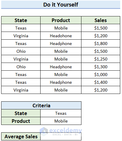
Practice Section
Here, I have provided a practice sheet for you to practice how to fix the AVERAGEIFS Value (#VALUE!) error in Excel.
Download Practice Workbook
You can download the practice workbook from here.
Conclusion
In this article, I tried to cover how to fix AVERAGEIFS Value (#VALUE!) error in Excel. Here, I explained 3 different reasons with solutions. I hope this article was helpful to you. Last but not the least, if you have any questions feel free to let me know in the comment section below.
Related Articles
- Difference Between AVERAGEIF and AVERAGEIFS in Excel
- AVERAGEIFS for Multiple Criteria in Different Columns in Excel
- How to Use AVERAGEIFS Between Two Values in Excel
- AVERAGEIFS Function with “Not Equal to” Criteria
- How to Apply AVERAGEIFS Function Between Two Dates in Excel
<< Go Back to Excel AVERAGEIFS Function | Excel Functions | Learn Excel
Get FREE Advanced Excel Exercises with Solutions!
