In this tutorial, I am going to show you 2 examples of how to use AVERAGEIFS between two values in Excel. You can quickly use these methods even in large datasets to find the average of any type of value. Throughout this tutorial, you will also learn some important Excel tools and functions that will be very useful in any Excel-related task.
How to Use AVERAGEIFS Between Two Values in Excel: 2 Examples
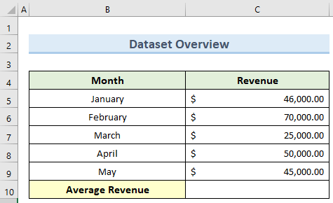
We have taken a concise dataset to explain the steps clearly. The dataset has approximately 6 rows and 2 columns. Initially, we formatted all the cells containing dollar values in Accounting format. Initially, we have 2 unique columns which are Month and Revenue. Although we may vary the number of columns later on if that is needed.
1. Using Single Range
We can specify a range for a single column inside the AVERAGEIFS function in Excel to calculate the average between two values. Follow the steps below to achieve this.
Steps:
- First, go to cell C10 and insert the following formula:
=AVERAGEIFS(C5:C9,C5:C9,">=46000",C5:C9,"<=70000")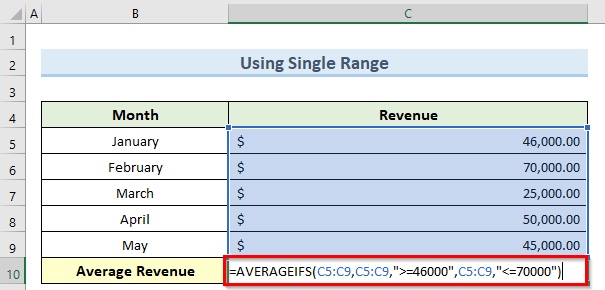
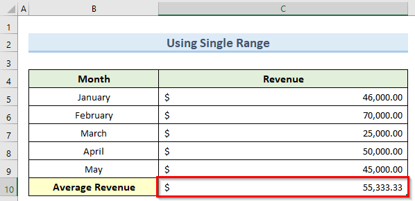
- Now, press Enter and this will calculate the average revenue only for the months that we entered in the range.
Read More: Excel AVERAGEIFS with Multiple Criteria in Same Range
2. Specifying Multiple Range
The AVERAGEIFS function in Excel gives the option to insert multiple ranges in order to find the average based on specific criteria. Note that, we have changed the column 1 title from Month to Month Number so as to include the numbers inside the formula. Let us see how to apply this function with multiple ranges.
Steps:
- To begin with, double-click on cell C10 and enter the below formula:
=AVERAGEIFS(C5:C9,B5:B9,">=1",B5:B9,"<=3")
- Next, press the Enter key and you should get the average revenue only for the months 1, 2, and 3 as we specified.

Read More: How to Use AVERAGEIFS Function for Multiple Columns
How to Use AVERAGEIFS Between Date Range
In many cases, we might need to find the average of input values within a certain date range. For example, we might want to calculate the average revenue for certain months and not all of them. Luckily, the AVERAGEIFS function in Excel can take date format values as criteria. You can enter the dates in any one of the valid date formats inside excel. Follow the steps below to apply this method.
Steps:
- To begin this method, double-click on cell C10 and insert the formula below:
=AVERAGEIFS(C5:C9,B5:B9,">=31-Jan-2021",B5:B9,"<=31-Mar-2021")
- Next, press the Enter key and consequently, this will find the Average Revenue for the input range of dates inside cell C10.

Read More: How to Apply AVERAGEIFS Function Between Two Dates in Excel
Things to Remember
- If you do not enter the minimum number of criteria or the average_range argument is a text value, you might get an #DIV0! error although you can see this error for some other reasons as well.
- This function will consider any empty cells as having a value of 0.
- All the input ranges must be of the same dimension.
- We can insert wildcard characters like ? and * inside this function.
- Remember to enclose the date criteria inside double quotes otherwise, the formula might not work.
- The AVERAGEIFS function will count only the cells that fulfill all the set criteria.
Download Practice Workbook
You can download the practice workbook from here.
Conclusion
I hope that you were able to apply the methods that I showed in this tutorial on how to use AVERAGEIFS between two values in Excel. As you can see, there are quite a few ways to achieve this. So wisely choose the method that suits your situation best. If you get stuck in any of the steps, I recommend going through them a few times to clear up any confusion. If you have any queries, please let me know in the comments.
Related Articles
- How to Use Excel AVERAGEIFS Function with Multiple Criteria
- [Fixed!] How to Fix AVERAGEIFS Value (#VALUE!) Error in Excel
- Difference Between AVERAGEIF and AVERAGEIFS in Excel
- AVERAGEIFS Function with “Not Equal to” Criteria
- AVERAGEIFS for Multiple Criteria in Different Columns in Excel
<< Go Back to Excel AVERAGEIFS Function | Excel Functions | Learn Excel
Get FREE Advanced Excel Exercises with Solutions!
