Latest Posts From Osman Goni Ridwan

Dataset Overview Suppose you have a dataset containing the sales quantity of two products over six months, and you want to create a bar chart based on this ...

Dataset Overview When working with data in Excel, you might need to create a chart that displays two different sets of values on separate X-axes. For ...

Dataset Overview Suppose you have a dataset with daily wages and sales data. You want to format the wages column using a color scale based on the sales value. ...

If you are looking for some easy and effective tricks to make a personal expense sheet in Excel then you are in the right place. Every person must track ...

Method 1 - Exiting and Restarting Excel to Turn Off Safe Mode You can simply close Excel and restart it and it's possible that Safe Mode is turned off ...

What Is Accrued Vacation Time? Generally, employees get a certain amount of days to leave for vacation, personal reasons, or sickness. But if the employee ...

Creating an operating budget in Excel may become time-consuming or daunting work. You don’t have to be a professional accountant or analyst to create an ...
Example 1 - Use the Consolidate Function for Text Data from Multiple Worksheets with the Power Query Tool Make sure all worksheets have the same rows and ...

Often, we get a list of addresses in a column, and we need to separate them into street addresses, city, state, and ZIP codes. So, you may want to learn how to ...

Method 1 - Group Time by Hour Intervals Go to the Insert tab in the top ribbon. Click on the Pivot Table option. Select the data from the ...

Method 1 - Create a Spin Button in Excel Step 1: Insert a Spin Button You have to enable the Developer tab. Go to Developer tab > Insert menu. ...

Method 1 - Use Filter Command Steps: Select the column where you want to apply the filter. Go to the top ribbon and select the Sort & Filter Tab. ...

Basic Elements of a Tally Sales Invoice Format Company logo and name Contact tetails Date, Invoice Number, and due date (If required) ...

Formulas for Horizontal Cylindrical Tank Volume Calculator The volume of a cylinder can be of two types: fully and partially filled. Partially filled volume ...

Step 1- Create a List of Products in Excel Create a new worksheet and enter the product list, the product code and its price. Select the cells to ...
- « Previous Page
- 1
- …
- 3
- 4
- 5
- 6
- 7
- Next Page »
See Our Reviews at


Hi Paulie,
Thanks for your comment. The VBA code is working completely fine from our end. Can you please share your workbook (.xlsm) file so we can check and find out the error easily?
Regards
ExcelDemy Team
Hi John,
Thanks for your comment. Follow the below procedures for your purpose:
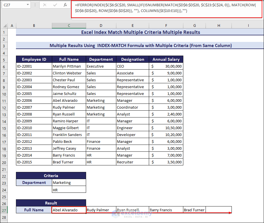
1. Get Multiple Results Using INDEX-MATCH Formula Based on 2 Criteria from the Same Column
Insert the following formula for the same case given in the article but to get values horizontally. After inserting formula in cell C27, drag the fill handle icon till it gives blank results.
=IFERROR(INDEX($C$6:$C$20, SMALL(IF(ISNUMBER(MATCH($D$6:$D$20, $C$23:$C$24, 0)), MATCH(ROW($D$6:$D$20), ROW($D$6:$D$20)), “”), COLUMNS($E$10:E10))),””)
2. Get Multiple Results Using INDEX-MATCH Formula Based on 2 Criteria from Different Columns
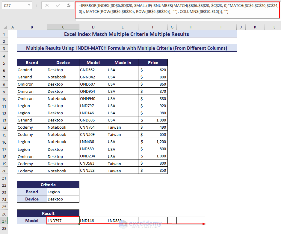
Similary for getting multiple results based on 2 criteria from different columns for same case given in the article but in horizontal direction, insert the following formula in cell C27 and drag the fill handle icon till it gives blank results.
=IFERROR(INDEX($D$6:$D$20, SMALL(IF(ISNUMBER(MATCH($B$6:$B$20, $C$23, 0)*MATCH($C$6:$C$20,$C$24,0)), MATCH(ROW($B$6:$B$20), ROW($B$6:$B$20)), “”), COLUMNS($E$10:E10))),””)
You can download the modified workbook from this link for your purpose. Hope, your problem will be solved. If not, share with us in the reply or you can share your workbook in ExcelDemy Forum.
Best Regards,
ExcelDemy Team
Hi Sue,
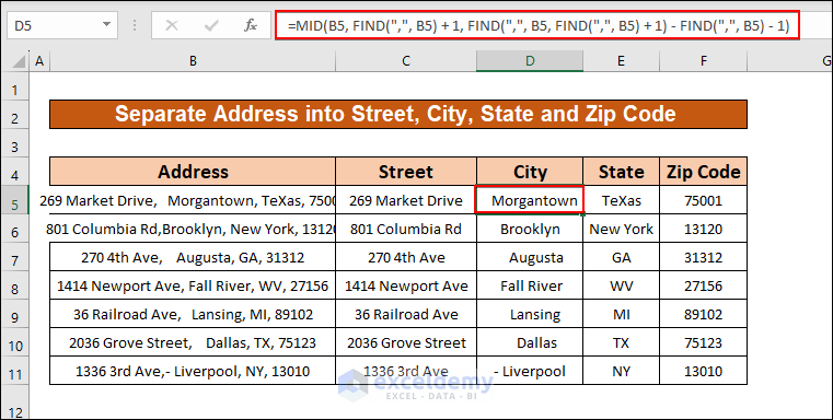
Thanks for your comment. In the formulas given in the article to retrieve the City name, we used SUBSTITUTE to remove extra spaces, find the position of the first comma, and extract the city name using the MID function. Also, we had to insert the length of the city name manually. If you want to make it dynamic, you can use the following formula in cell D5:
Dynamic Formula to Retrieve City Name from Full Address:
=MID(B5, FIND(“,”, B5) + 1, FIND(“,”, B5, FIND(“,”, B5) + 1) – FIND(“,”, B5) – 1)
This formula finds the position of the 1st and 2nd commas and extracts all characters between them to get the city name.
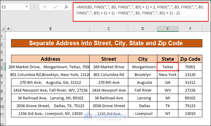
And for state names, we have used formula to retrieve only those in the abbreviated formats. If you want to get state names in full forms, then use the given formula:
Dynamic Formula to Retrieve Full State Name from Full Address:
=MID(B5, FIND(“,”, B5, FIND(“,”, B5) + 1) + 2, FIND(“,”, B5, FIND(“,”, B5, FIND(“,”, B5) + 1) + 1) – FIND(“,”, B5, FIND(“,”, B5) + 1) – 2)
Using this formula, you will get all characters between the 2nd and 3rd comma. Thus you will get the state name in full form.
Hope, your problem will be solved. If not, share with us in the reply or you can share your workbook in the ExcelDemy Forum.
Best Regards,
ExcelDemy Team
Hi KIEL,
Thanks for your question. Actually, you may seem that the choice of using prior year prices for Volume Variance and current year volumes for Price Variance is wrong, but it aligns with certain assumptions and conventions often used in variance analysis. Let me explain the reasoning behind this choice:
1. Volume Variance based on Prior Year Price:
The assumption here is that changes in quantities sold are evaluated against the prices of the prior year. Volume Variance assesses the impact of selling more or fewer units than planned at the prior year’s prices. Using the prior year’s price isolates the impact of changes in quantity sold, assuming that the pricing structure from the prior year remains relevant.
2. Price Variance based on Current Year Volume:
Here, we’re checking how price changes between this year and last year affect earnings, considering the amount sold this year. We assume that this year’s sales volume reflects the current business situation, and any price changes are looked at based on this year’s sales.
I think you have understood the matter. If you have any further queries please inform us in the reply.
Warm Regards,
ExcelDemy Team
Hi Strike,
Thanks for your comment. The Mix Variance formula provided in the article is based on Revenue rather than Quantity because it is intended to capture the impact of changes in the sales mix of different products on revenue, which includes both price and quantity components. Here’s the formula:
Mix Variance = Revenue PY * (Price PY – Average Price PY) * Mix Change / 100
By using Revenue PY in the formula, you are considering both the price and quantity component. Thus it becomes a comprehensive way to evaluate how the mix of products contributed to changes in revenue. It provides a more complete picture of why the revenue changed. Using Quantity alone would only consider the quantity component and not account for price changes, which are also crucial in understanding revenue variations.
If you have any further query, then please inform us in the reply section.
Regards,
ExcelDemy Team
Hi BP,
Thank you for your comment. To solve the sequencing problem, you may go through these two articles,
1. Solving Sequencing Problems Using Excel Solver Solution
2. Sequencing problem using Johnson’s algorithm of scheduling n-jobs on 2-machines
Please go through these articles. If you have any further queries then please inform us in the reply.
Thanks and regards,
ExcelDemy Team
Hi Harrison,
Thanks for your comment. Calculating the probability of success of a project is actually a complex task that depends on various factors. One common approach is to use a weighted scoring system based on certain criteria for each project. Here’s a simplified template you can use:
Step 1: Define Criteria and Assign Weights
=>> Create a list of criteria that are important for determining the success of a project. These criteria may include factors such as budget, timeline, team expertise, market demand, and alignment with strategic goals.
=>> Assign weights to each criterion to reflect their relative importance. For example, if the timeline is more critical than the budget, you might assign a higher weight to the timeline criterion.
Step 2: Evaluate Each Project
=>> Assess each project in your portfolio against the defined criteria. You can use a scale (e.g., 1 to 10) to rate each project’s performance on each criterion.
=>> Multiply the ratings by the assigned weights for each criterion and calculate the weighted score for each project.
Step 3: Calculate Probability of Success
=>> Add up the weighted scores for each project to get a total score. The total score represents the overall potential for project success.
=>> You can then convert this total score into a probability of success. This step is somewhat subjective, and you might need to set specific thresholds for what constitutes a “high probability of success“. For example, you could establish that a total score above a certain threshold (e.g., 80 out of 100) indicates a high probability of success.
=>> You may want to use historical data or expert judgment to help determine the relationship between total scores and success probabilities.
Finally, you can express the probability of success as a percentage. For instance, if a project has a total score of 85 out of 100, and this is associated with a high probability of success, you could say that the project has an 85% chance of success.
Hello Nivedita,
Thanks for your comment. Here, “112500” represents the tax amount to be added to the calculated TDS when the annual salary income (C11) exceeds 1,000,000 (1 million) and falls within the highest tax slab.
To break it down further:
>> If the annual salary income (C11) is greater than 1,000,000, it means that the individual’s income falls into the highest income tax slab.
>> In this highest tax slab, the formula applies a tax rate of 30% to the portion of income above 1,000,000. It calculates the tax on this portion and adds 112,500 to the result.
Inform us in the comment if you have any more confusion.
Regards,
ExcelDemy Team
Hello Komal!
Thanks for your comment. I see that you are facing some troubles while running the Date Picker UserForm macro. As you have created some more text boxes so I have the following suggestion that you should check:
>> Check that all the textboxes should be inside one UserForm. Also, check whether all the macro codes are written for the same UserForm or not. They all must be under same UserForm to be run properly.
If still you are facing issue then please send us your workboook for this you can post it the ExcelDemy Forum. As the file is working completely fine from our end, it is necessary to have your workbook to find the error.
Regards
Hi Ketayla!
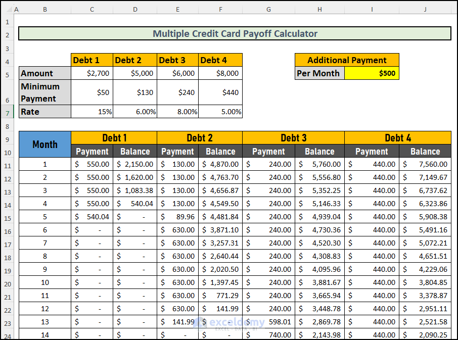
Thanks for the comment. There were some errors in the formula of Lowest Debt Calculation and I have fixed it. Also for your convenience, I have added the debt 4 in the workbook. Following the same method, you can create a formula yourself for debt 5, debt 6, and more. You can download the file from this link.
Here is the image of the solution:
Thanks for supporting us! If you face any other problem with any other topic then reply in the comment section.
Hello Ankit,
Thanks for sharing your problem. The file is working completely fine from our end. So, if you think your Excel VBA function is not working after saving and reopening the workbook, there could be several reasons for this issue. Here are some common troubleshooting steps to help you resolve the problem:
1. Check for Macro Security Settings:
>> Excel has a security feature that may disable macros by default.
>> Make sure that macros are enabled in your Excel settings.
>> Go to “File” > “Options” > “Trust Center” > “Trust Center Settings.” Under “Macro Settings,” select “Enable all macros” or “Enable macros for this session” to allow macros to run.
2. Check Workbook FIle Extension
Check if the VBA code is stored in a macro-enabled workbook (with the .xlsm file extension) rather than a regular .xlsx workbook. Macros won’t run in regular Excel workbooks.
3. Check Event Triggers:
Check that we have used the code associated with each worksheet. Make sure that these events are still properly associated with the worksheets in your file.
I believe by following these steps, you should be able to identify and resolve the issue. Please inform us of the outcome in a reply. Thanks for staying with us!
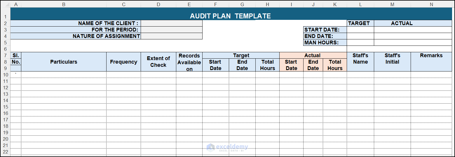
Hello AM!
Thanks for your comment. To schedule the audit workload and assign resources, you can create an Audit Plan Template. To do this, you have to assign these parameters. I am listing the items with proper descriptions:
1. Particulars: This column should describe the specific audit item or task that needs to be checked or reviewed. It could be a process, financial statement, or any other aspect of the audit.
2. Frequency: This column specifies how often the particular item is audited. For example, it might be done annually, quarterly, monthly, or as needed.
3. Extent of Check: This column outlines the depth or scope of the audit procedure. It could be a high-level review or any other specified level of scrutiny.
4. Records Available On: This column indicates where the relevant records or documents are available. 5. Target Start and End Date: These columns define the planned dates for starting and completing the audit procedure for the particular item.
6. Actual Start and End Date: These columns record the actual dates when the audit procedure for the specific item started and ended.
7. Total Hours: This column can be used to record the total number of hours spent on auditing the particular item.
8. Staff’s Name: This column mentions the name of the staff or auditor responsible for conducting the audit for the particular item.
9. Staff’s Initial: This column can be used for the staff member’s initials or code for identification purposes.
10. Remarks: This column allows auditors to provide comments or notes related to the audit of the specific item. This can include observations, findings, issues, or any other relevant information.
Here, you can see the image of the template that I have made for you. Also, you can download the template from the following link.
Hello AMIR,
Hope you are doing well and thank you for your query. You can extract comments from word document with their respective locations in an Excel sheet. For this, you can use the following code:
Sub ExtractCommentsFromWordToExcel()
Dim cmt As Comment
Dim j As Long: j = 1
Dim xAPP As Excel.Application
Dim xWB As Excel.Workbook
Set xAPP = CreateObject(“Excel.Application”)
xAPP.Visible = True
Set xWB = xAPP.Workbooks.Add
With xWB.Worksheets(1)
For Each cmt In ActiveDocument.Comments
.Cells(j, 1).Value = cmt.Range.Text
.Cells(j, 2).Value = “Page ” & cmt.Scope.Information(wdActiveEndPageNumber) & “, Section ” & cmt.Scope.Sections(1).Range.Information(wdActiveEndSectionNumber)
.Cells(j, 3).Value = Format(cmt.Date, “dd/MM/yyyy”)
j = j + 1
Next cmt
End With
Set xWB = Nothing
Set xAPP = Nothing
End Sub
Here is an image displaying the result in Excel sheet:
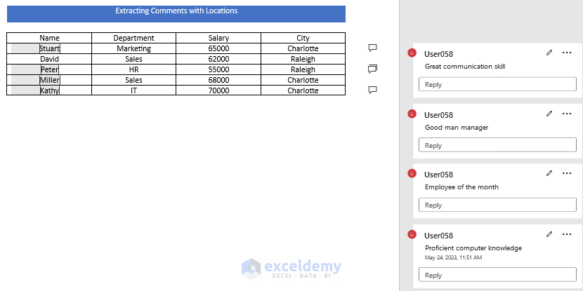
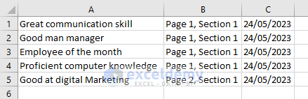
Hope you find this useful. Have a good day. Please let us know if you have any further queries. Also, you can post your Excel-related problems in the ExcelDemy Forum with images or Excel workbooks.
Hello MATT!
Thanks for the comment. Mistakenly I forgot to insert the VBA code in the article but now I have corrected it and added the VBA code in the article so it will be helpful for the readers to use in their workbooks.
Thanks again. Please, browse ExcelDemy blogs for more Excel related problems. Also you can take help for your Excel related problems by posting it in our ExcelDemy Forum with your workbooks.
Regards
Osman Goni Ridwan
Hello ANDREW,
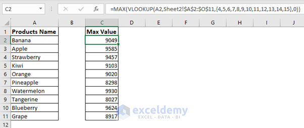
Hope you are doing well and thank you for your query. You can use VLOOKUP and MAX functions among other methods to look for a value when the value you want to analyze for is in columns D through O.
You can use the following formula.
=MAX(VLOOKUP(A2,Sheet2!$A$2:$O$11,{4,5,6,7,8,9,10,11,12,13,14,15},0))You can find the solution to your problem in the Excel file linked to this reply.
VLOOKUP and MAX to Look for Max Value
Regarding your query of product names changing in accordance with your changing the names in Sheet 1, you can use cell reference to copy the product names in Sheet 2. This will look for the correct row of data in Sheet 2.
Here is a screenshot of the results in the Excel file.
Hope you find this useful. Have a good day. Please let us know if you have any further queries. Also, you can post your Excel-related problems in the ExcelDemy Forum with images or Excel workbooks.
Regards,
ExcelDemy Team
Hello BUAN,
The Data Types option is not available for Excel 2019 version.
It is only available for Excel for Microsoft 365, Excel for Microsoft 365 for Mac, and Excel for the web.
You need to buy a subscription to Microsoft 365 to use these options.
If you have any further queries, kindly post them on our Exceldemy Forum.
Regards
Exceldemy Team
Hello FELICIA SANTOS,
I hope you are doing well! Here, I have created a dataset as you have described and calculated the total amount spent per category.
>> Here, you have to insert the name of the category in cell F5.
>> Then, insert the following formula into cell G5:
=SUMPRODUCT(D3:D10*(C3:C10=F5))Thus, you will get the sum of the amount as per the selected category.
I hope, your problem will be solved in this way. You can share more problems in an email at [email protected]
Hello JULIO!
Hope you are doing well. In our dataset, Method 7 is working properly without any errors. If you are facing errors, that can be for the following reasons:
1. If any cells that are used in the TEXTJOIN function exceed 252 characters.
2. If the output of the TEXTJOIN function exceeds 32672 characters which is the cell limit in Excel.
3. And, sometimes Excel fails to identify the delimiter as text. For this, you should use delimiters inside the inverted commas and shouldn’t use the CHAR functions to generate any symbols.
I hope, your problem will be solved in this way. You can share more problems in an email at [email protected]
Hello BRYAN!
As per your question, I have added a new portion in the article which contains the method how you can calculate the accrued time after the completion of probationary period automatically.
I hope, your problem will be solved in this way. You can share more problems in an email at [email protected]
Hello ALLISON!
you can use the “Use of SUMIF with INDEX-MATCH Functions to Sum under Multiple Criteria” method for your problem. Here, we have used the brand name as criteria and you can substitute it by Year. See this screenshot below:
While using this method, you have to fill in both criteria. So, you must put both the year’s and month’s values.
I hope, your problem will be solved in this way. You can share more problems in an email at [email protected]
Hello JUSTINA!
I have an easy solution to your problem. To copy data of range Sheet1 (A10072:AT10801) to range Sheet 2 (A10772:AT10801), you can use this VBA Code.
And to copy data of range Sheet 1 (A10802:AT10831) to the range Sheet 2 (A10802:AT10831), use the following VBA code-
I hope, your problem will be solved in this way. You can share more problems in an email at [email protected]
Hello YINKA! I am very glad to hear that this article has helped you. You will find many more Excel-related articles on ExcelDemy. also, You can share your Excel-related problems with us to get a solution. Send an email at [email protected]
Thank You!
Hello BORIS!
You can try to “Multilayer Pie Chart” or “Bar of Pie chart” to solve your problem. You can follow this article to create these types of pie charts for your dataset. Please, go through this article,
How to Make a Multi-Level Pie Chart in Excel
I hope, your problem will be solved in this way. You can share more problems in an email at [email protected]
Hello ISH SHARMA!
You can increase and decrease decimal digits from the format options. But Through this, it will round to the nearest decimal. Suppose, when you round the value 44.41, it will be rounded to 44.4, not 44.5 and for the value 44.45, it will become 44.5.
To use this method,
>> Select the cell.
>> Go to the Home tab in the top ribbon.
>> Here, in the Number menu, click on the “Increase Decimal” icon to increase the decimal digits after the point, and click on the “Decrease Decimal” to decrease the decimal digits.
I hope, your problem will be solved in this way. You can share more problems in an email at [email protected]
Hello N R RAVINDREA!
Thank you for your suggestion. We are taking this into concern. And, You can share your Excel-related problems in an email at [email protected]
Thank You!
Hello YINGYANG!
Syntax of IF function is as follows: =IF(logical_test, [value_if_true], [value_if_false])
So, for the formula
=IF(B2="",NOW(),B2):>> logical_test – B2=”” : It is the condition of the IF function. The condition is when cell B2 is blank.
>> value_if_true – NOW() : This is the output when the cell meets the logical test. The NOW() function gives the present time in the cell.
>> value_if_false – B2 : When the cell will not meet the criteria, the IF function will return the cell value of B2.
So, in brief, when cell B2 is empty, the formula will insert the present time in the cell; if it isn’t empty, it will leave the cell as it is.
I hope, your problem will be solved in this way. You can share more problems in an email at [email protected]
Thank You!
Hello ARIF, to get the dates in the next row use the following code when you will insert values in cells of range B3:I3 and want to auto-populate date and time in cell range B4:I4.
CODE:
You can change the cell range as your want. I hope, your problem will be solved in this way. If not, please share the Excel file and send us the problem with a little more explanation in an email at [email protected]
Hello ABBY!
You have to change a line in the VBA code that is defining the format of the output.
Insert this line:
.NumberFormat = “dd mmm yyyy” instead of this .NumberFormat = “dd mmm yyyy hh:mm:ss”
So, the code will become as follows-
Hello BEN!
I think the solution to your problem is already solved in method 1 of this article. To search for partial match, you have the wild cards (*) that have been shown in method 1.
If the cell C13 contains the value of the search item. Then use the following formula:
=VLOOKUP(“”&C13&””,$B$4:$C$11,2,FALSE)
I hope, your problem will be solved in this way. If not, please share the Excel file and send us the problem with little more explanation in an email at [email protected]
Thank You!
Hello RJ LENNOX!
In method 1.3m there have been shown only the formula for the names of the right order and in previous methods, there has been shown formula to get the value of CGPA in the right order. Please insert this formula into cell F7:
=LARGE($C$5:$C$14,ROWS($F$7:$F7))and, drag the fill handle to get the top 5 cgpa values.
I hope, your problem will be solved in this way. If not, please share the Excel file and send us the problem with a little more explanation in an email at [email protected]
Thank You!
Thank you, BOKEP. Thank you for your comment. Read more articles on Exceldemy and share them with your friends and family. Keep supporting us!
Hello AVINASH! I have made a dataset as per your description and solved your problem. You can paste the following formula into the column O and the 3rd row to get the comment from sheet 1 when the criteria are met:
Try this for your dataset and let us know the outcome. Thank You!
Thank you! Shakeel. We are really honored to hear that our articles have helped you. Browse articles of Exceldemy more and share with your friends and family and keep supporting us!
hello, EMIN! Actually, I haven’t understood what you asked in this comment. Can you please mail us the problem with a little more explanation at this address: [email protected].
We will try our best to solve your problem. thank You! And, keep browsing Exceldemy.
Hello M LAVI! with this code, only the column of the active cell that contains the target cell value will be hidden.
And, you can copy and paste the drop-down cell to other worksheets without assigning data validation again. If you have anything more to know then inform us in a comment!
Hello JUSTIN! The code is working perfectly from my side and the output has been shown in the practice workbook. And, it is not necessary to add code “Dim Cell as Range” here as we are not working with the cell value. But it is a good practice to declare variables at first.
We have a large collection of Excel-related blogs that will help you to solve many more problems. Browse them and let us know your opinion in the comment section. Thank You!
Hello SHAWN S FAHRER!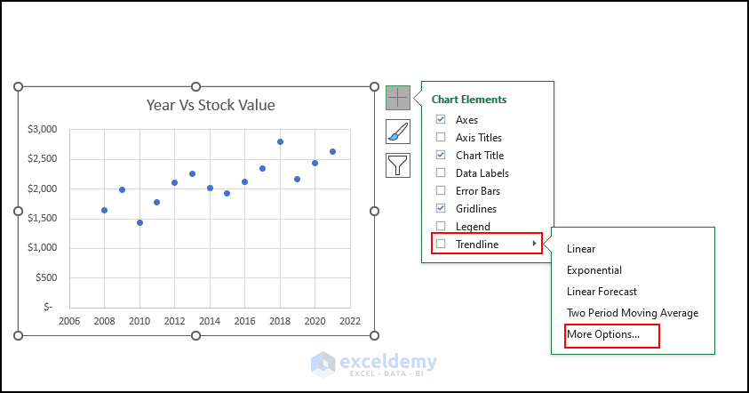
You can get a quadratic equation from a graph with a few points that you have mentioned here. Follow the steps below for this
First, create a graph with the points you have.
Then, Go to the Chart Elements clicking the Plus icon.
Click on the arrow beside the “Trendline” option.
Go to the “More Options”
1
Here, you will go to a window named “Format Trendline”.
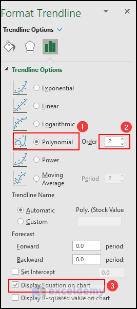
Select the “Polynomial” option of order 2.
Mark the checkbox saying “Display Equation on Chart”.
As a result, you will there will create a trend line following a quadratic equation which is also shown in the graph.
Try this method and let us know the outcome! Thank You!
Hello MANUJ! You have to insert a value as the set value for cell G3 to use Goal Seek feature.. suppose you have an equation like 5x^3 – 2x^2 + 3x – 21 = 0 then you can change the equation like 5x^3 – 2x^2 + 3x – 6 = 15. Here, we have done this.
And, yes! you are right that the cubic function gives 3 root values. But using the Goal Seek Feature, you will get only one root. and, in many times, the cubic function may have one real root and 2 complex roots. In these cases, the goal seek feature will give the value of the real root.
Try these examples and let us know the output. Thank You!
Hello, JACK! For this, you have to add a new conditional Formatting rule. Go to Home tab >> Conditional Formatting >> New Rule.
Then, Select the “Format Only Cells That Contain” and select the “Blanks” option in the “Format only cells with” box.
Then, go to the “Format” option and select White as the fill color.
Try this and let us know the outcome. Thank you!
Hello JUILA! I hope you are fine. You can easily create a conditional drop-down list from other worksheets in the same workbook. You can follow this article-
https://www.exceldemy.com/excel-drop-down-list-from-another-sheet
This article will show you the process step-by-step with proper illustrations. Try the methods mentioned in this article and let us know the outcome. Thank you!
Hello APRIL, We already have an article written based on your problem. I hope, you will find this helpful. Follow this link below-
https://www.exceldemy.com/excel-vlookup-multiple-criteria-without-helper-column/
Try the methods mentioned in this article and let us know the outcome. Thank you!
Hello Roy! Thank you for your comment. I must say your knowledge of Microsoft Excel is really appreciable. Keep commenting on posts of Exceldemy and help others to learn more.
Hello Johan, you can use the following procedure to serve your purpose-
– Make a column with 101, 102, 103, and so on.
– Make a column with A, B, C, D, and repeat.
Follow this article to repeat numbers or characters serially.
How to Add Numbers 1 2 3 in Excel
– Then use CONCATENATE function to combine them.
Let us know the outcome in the reply. Thank you!
Hello Nasser Enami, you can follow this article to solve your problem.
https://www.exceldemy.com/separate-address-in-excel-with-comma
In this article, you will find how to separate an address into a city, state, and zip code using an Excel formula. You can modify this file for your purpose. In your dataset the separator is “|” and you have to use 3 separators. Modify this worksheet as shown in the screenshot below-
Let us know the outcome in the reply. Thank you!
hello, you can use the FILTER function to do this. Suppose, you have inserted your dataset into the range B2:D6.
And, in cell G2. you have inserted the id for what you want to get month and payment.
so, to get the required data, you have to insert the following formula into any blank cell:
Use this formula for your dataset and let us know the outcome in the reply. Thank you!
Hello Ahmed, you can go through this article-
https://www.exceldemy.com/calculate-cost-per-unit-in-excel/
I hope, you will find your solution. Let us know the outcome by leaving a comment. Thank you!
Thank You, Roy, for your precious comment!
Hello Edward, to find out the total sales for one month, you can follow Criteria 7 of the following article.
https://www.exceldemy.com/sum-index-match-multiple-criteria-in-excel/
Here, the Criteria 7 shows how to determine the output based on all Rows & 1 Column with SUM, INDEX, and MATCH functions together. Let us know the result in the reply. Thank you!
Hello SONYA, you can face this issue because of the following reasons:
1. Incorrect Cell Ranges used in the formula
2. The Date format used in the formula is not correct. You have to use a similar data format both in the cells and formulas.
Check these things in your workbook and let us know the outcome. Thanks!
Hello SHANMUGAM, can you please explain your problem a bit more elaborately? Then it will be easy to help you. Thanks!
Hello Peter and Charlie, the solution described in this article at Criteria 2: “Extracting Data Based on 1 Row & 2 Columns with SUM, INDEX and MATCH Functions Together” is perfectly working from our end.
Just to inform you, you can’t use a cell reference in the Look_up value of the MATCH function instead you have to insert the single of multiple look_up values manually e.g. {“Feb”,”Jun”}. Hope you have found your solution. Try it and let us know the outcome in a reply. Thank you!
Hello, we are glad to hear that our article has helped you. After seeing your comment, I have extended the dataset to 260 rows and the formulas have worked perfectly from my end. Can you please recheck whether you have changed the formula text corresponding to your dataset? For example, in the dataset of 11 rows the formula for largest 5 values will be like
=LARGE($C$5:$C$14,ROWS($G$7:$G7))but when you extended the dataset till 260th row then the formula will be like
=LARGE($C$5:$C$260,ROWS($G$7:$G7)).If you still face the problem then inform us in the reply. Thank you!