Method 1 – Use Filter Command
Steps:
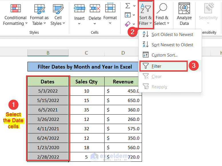
- Select the column where you want to apply the filter.
- Go to the top ribbon and select the Sort & Filter Tab.
- Click on the Filter option.
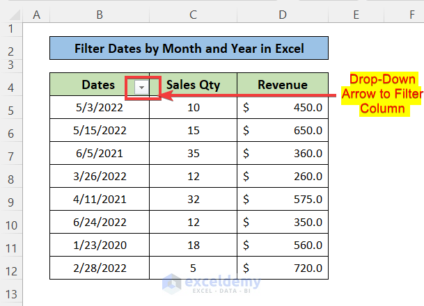
- You will see a drop-down arrow created in the Header cell of the column.
- Click on this to apply the filter.
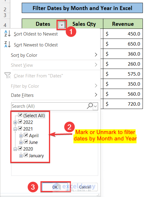
- After clicking, you will see the list of years and months in a new window.
- You can mark or unmark the options to apply a filter on the dates.
- By clicking on the Plus(+) icon on the left side of the years, you will open the list of months. You can click on the plus(+) icon on the left side of any month to open the day’s list.
- Mark the specific month and year to filter only for that month and year. Whereas, unmark the remaining boxes.
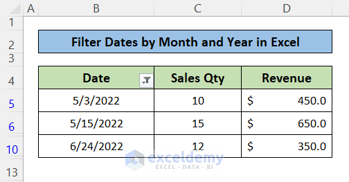
- If you check the year 2022 and the months of May and June from the filter list, you will get the filtered table as shown.
Method 2 – Apply Excel FILTER Function
You can use the Excel Filter Function to filter dates by months and years.
Steps:
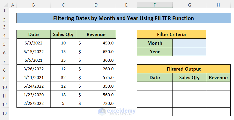
- Create a table “Filter Criteria” to collect input data of month and year.
- Make a table Filtered Output where you will get the output depending on the filter conditions.
- Enter the following formula into cell F10 to use the FILTER function to filter dates by month and years.
=FILTER(B5:D12,(MONTH(B5:B12)=G5)*(YEAR(B5:B12)=G6),"N/A")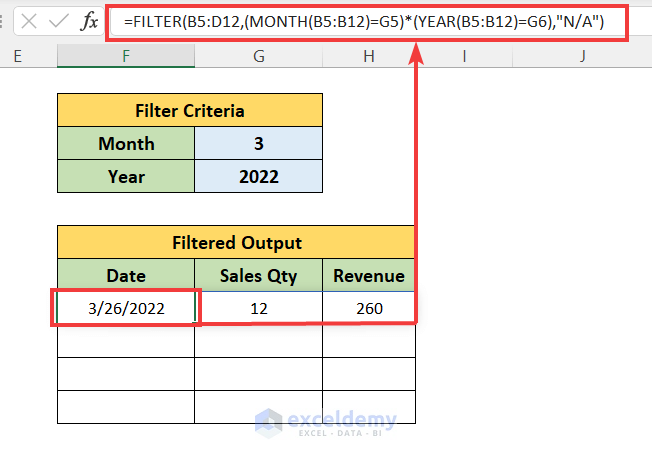
- Enter the value in the month and year cell.
- You will get the filtered output for the specific month and year.
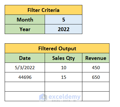
- You can enter the value of month and year in the specific cells to filter dates by month and year using the Filter Function.
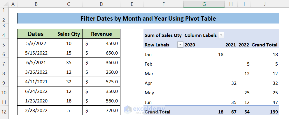
Method 3 – Utilize Excel PIVOT Table Tool
Steps:
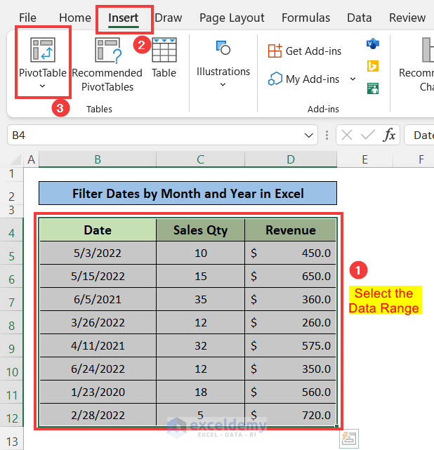
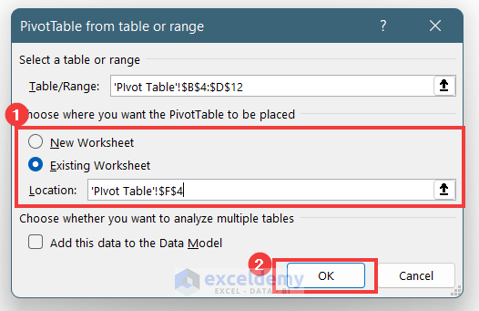
- Select the data range.
- Go to Insert > Pivot Table.
- Select the Existing Worksheet option and select a cell in the location box to specify where to start the pivot table.
- Press OK.
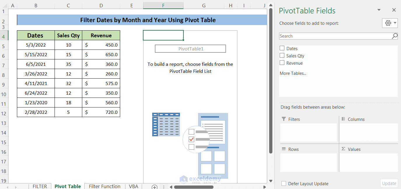
- You will see a pivot table box created from the cell you specified and a window named PivotTable Fields will be created on the right side of the worksheet.
- You will find the column names as a list.
- Drag the Dates option in the Rows box and the Sales Qty option to the Values box.
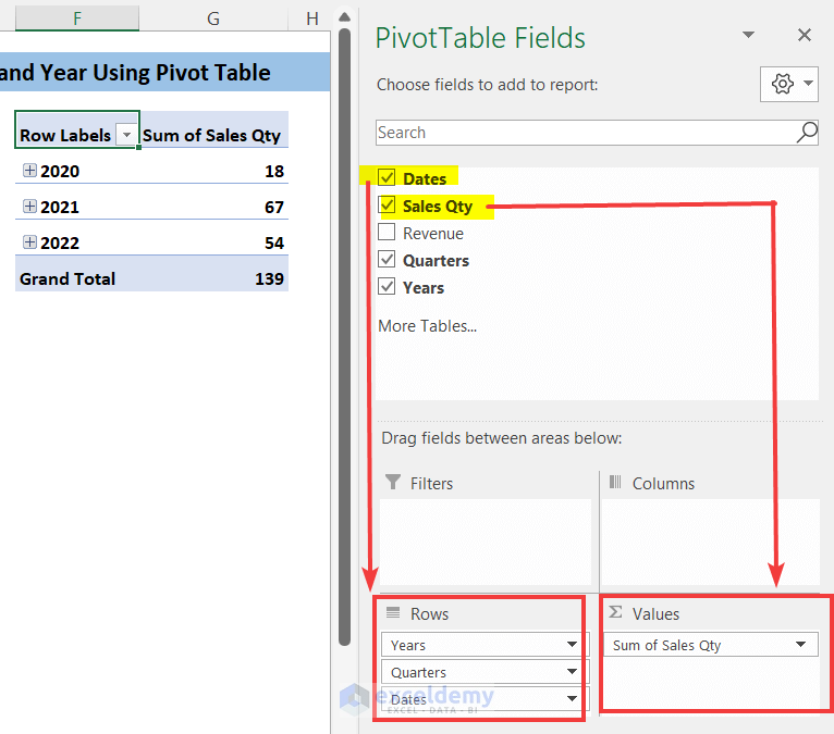
- Remove the Quarters option from the rows options.
- Move the Years option to the column box.
- You will see a perfect Pivot table where you can see the Sales Qty with months in Rows and Years in Columns.
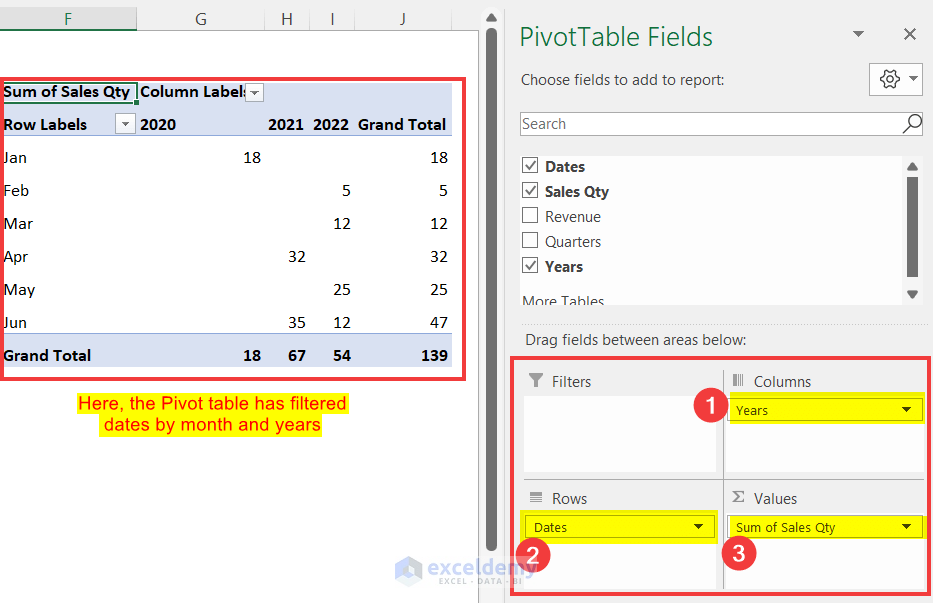
- The values are filtered by months and years.
- You can also specify a filter for month and year by clicking on the drop-down arrow on the cell Column Labels and Row Labels.
- Go to Column labels to select the Year and Row labels to select the Months.
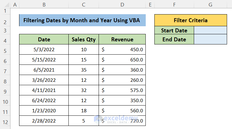
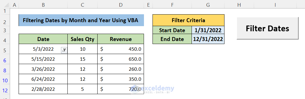
Method 4 – Create a Button with VBA to Filter Dates by Month and Year
Steps:
- Before entering the code, specify cells to insert the Start Date and End Date in the Filter Criteria box.
- If you want to filter dates for June 2022, you will give the Start date as of 06/01/2022 and the End Date as of 06/30/2022.
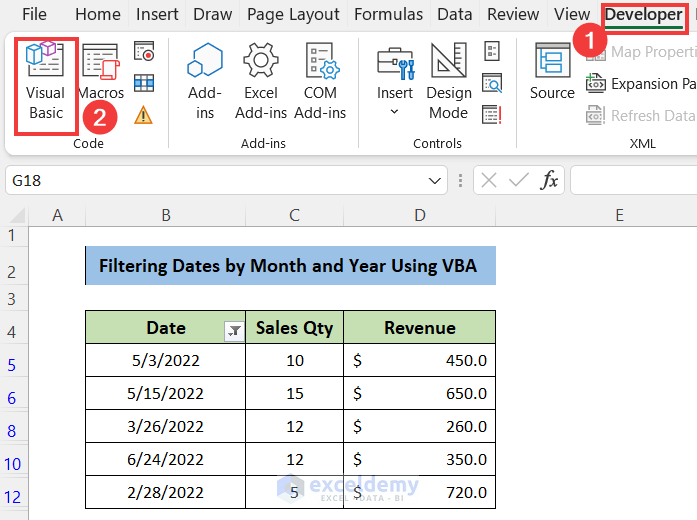
- Go to the Developer tab in the top ribbon. Click on the Visual Basic You can also use ALT + F11 to open the ‘Microsoft Visual Basic for Applications’ window if you don’t have the Developer tab added.
- The ‘Microsoft Visual Basic for Applications window will pop up. Click on the Insert option.
- Select Module from the option.
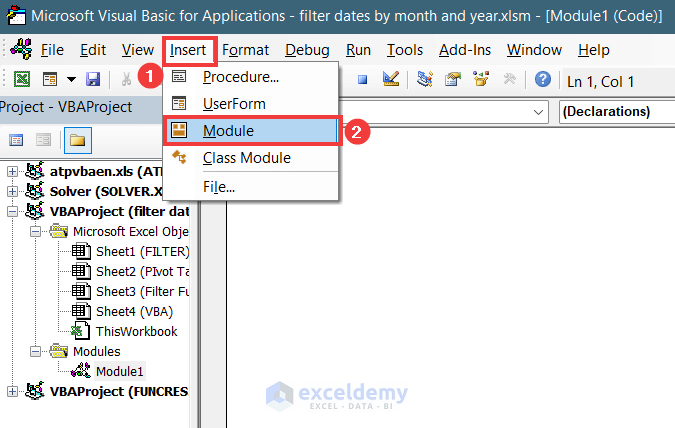
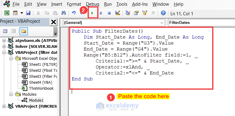
- A new ‘Module’ window will appear. Paste this VBA code into the box.
Public Sub FilterDates()
Dim Start_Date As Long, End_Date As Long
Start_Date = Range("G3").Value
End_Date = Range("G4").Value
Range("B5:B12").AutoFilter field:=1, _
Criteria1:=">=" & Start_Date, _
Operator:=xlAnd, _
Criteria2:="<=" & End_Date
End Sub
- To run the code, go to the top menu, press on the ‘Run’ option (shortcut key is F5).
Explanation of VBA Code:
- Public Sub FilterDates()
That creates a Macro named FilterDates
- Dim Start_Date As Long, End_Date As Long
Declares two-variable named Start_Date and End_Date and the format is Long
- Start_Date = Range(“G3”).Value
Taking the value of Start Date from the cell G3
- End_Date = Range(“G4”).Value
Taking the value of End Date from the cell G4
- Range(“B5:B12”).AutoFilter field:=1
Declaring the range of cells where to apply filter by VBA AutoFilter function. Here you have to input the range of your Dataset.
- Criteria1:=”>=” & Start_Date
Setting the condition of the filter for the dates which are greater than the start date.
- Operator:=xlAnd
Putting And operator to add another condition of filter which will apply AND logic.
- Criteria2:=”<=” & End_Date
Setting the condition of the filter for the dates which are less than the end date.
- End Sub
Declaring the end of the Macro
- You can add a Macro button so you don’t have to go to the module tab to run the code and filter.
- Go to the Developer tab > Insert and select the Button icon.
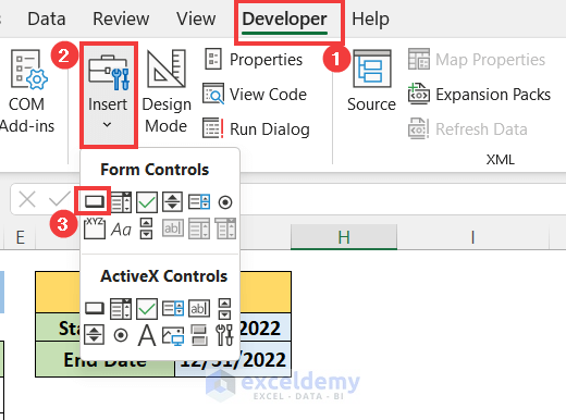
- Draw a box in the worksheet and label it.
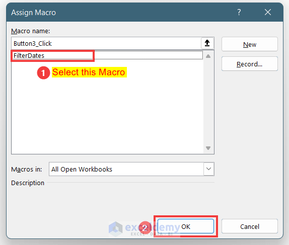
- Select the Macro from the list. Press OK.
- You can see that a Button has been created. Rename it to Filter Dates.
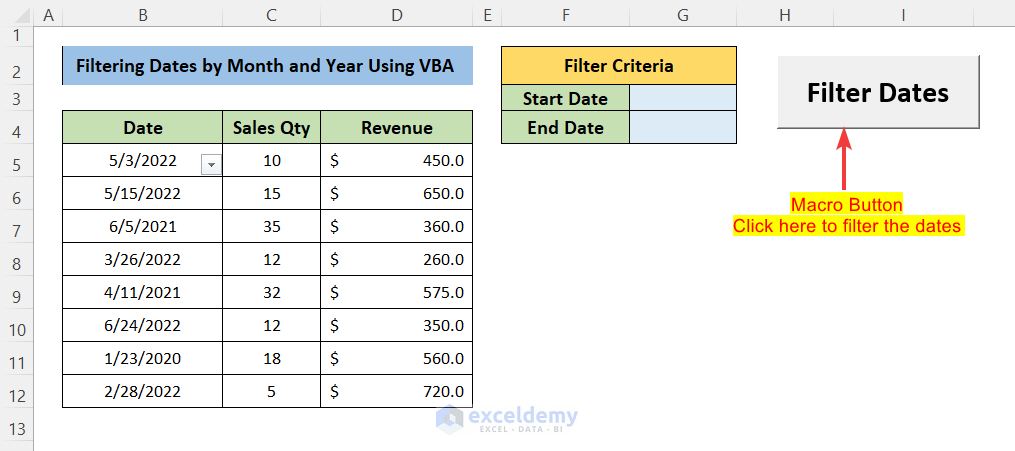
- Insert a Start Date and End Date in the cells to filter the dates by month and year then press the Macro button.
Things to Remember
- You must edit the data range in the VBA code before applying it to your dataset.
- The Excel Filter option is the easiest way to apply a filter but it changes the main dataset.
- Use the Filter function or Pivot Table to apply the filter if you want to keep the main dataset unchanged.
Download Practice Workbook
<< Go Back to Date Filter | Filter in Excel | Learn Excel
Get FREE Advanced Excel Exercises with Solutions!
