How to Group Dates by Filter in Excel: 3 Easy Methods

Method 1 – Using Filter Command to Group Dates by Filter in Excel

1.1. Utilizing AutoFilter Simply

Steps:

• Select any data or the entire dataset on your worksheet. Go to Editing > Sort & Filter > Filter.

Note: You can enable the AutoFilter option by pressing CTLR + SHIFT + L.

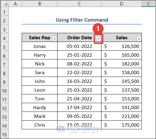
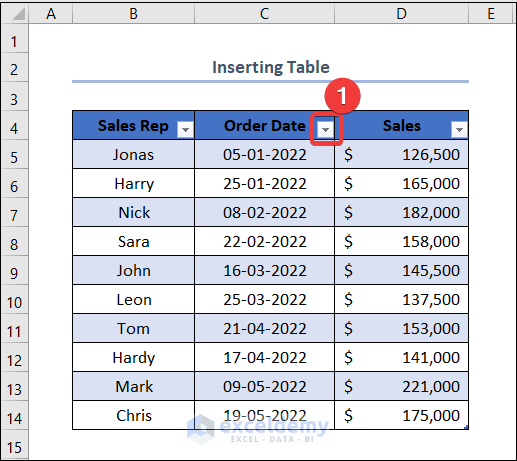
• The Filter option is now enabled, and the Filter icon can be found on the right side of each Header. Click the Filter icon in the Order Date Header to filter dates.

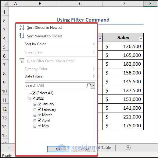
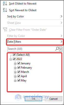
• You’ll see various options presented, such as the image below.

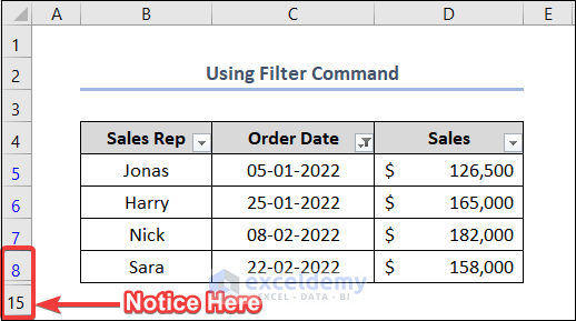
• Filter data only for January and February, check those boxes, uncheck the rest, and click OK.

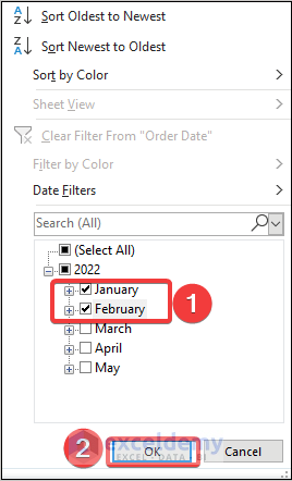
• Excel only displays data for January and February. Rows 9 to 14 are hidden because they don’t contain data from those months.

1.2. Applying Date Filters

Steps:

• Open the filter choices by pressing the Filter icon in the Order Date’s header, just as you did in the previous section. Choose Date Filters > Last Month.

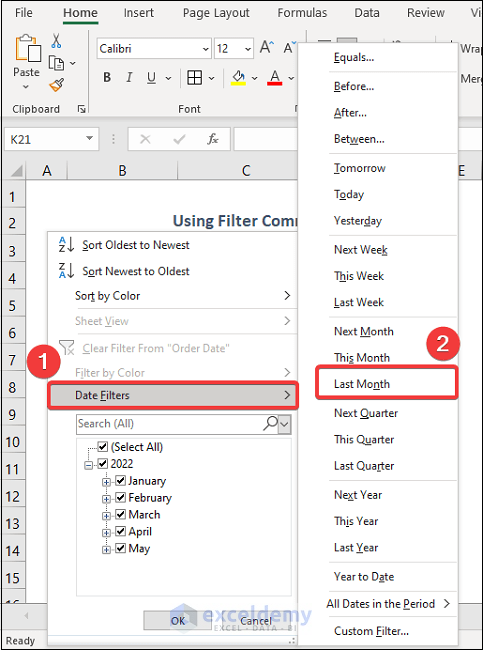
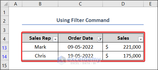
• It will show the filtered data for the last month. As it is June, data for May month will be shown here.

1.3. Implementing Custom AutoFilter Option

Steps:

• Click Date Filters > Custom Filters.

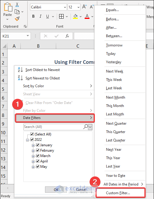
• A Custom Autofilter dialog box opens. The two boxes above are for the start date and the remaining lower two’s are for the end date. Fill up boxes sequentially like the picture below to get the data between 1 Feb to 31 May of the year 2022 and click OK.

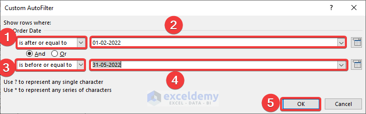
• Obtain all of the filtered data for the dates we’ve chosen.

Method 2 – Creating Table and Grouping Dates

Steps:

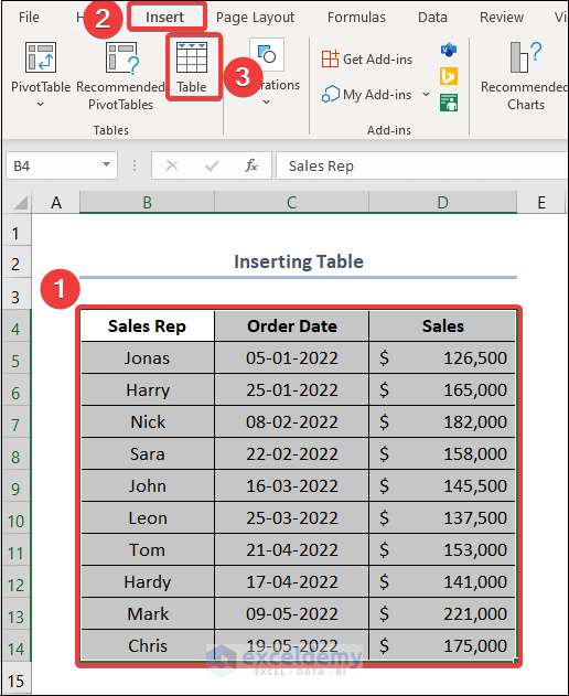
• Select the entire range of cells containing data. Select Insert > Table.

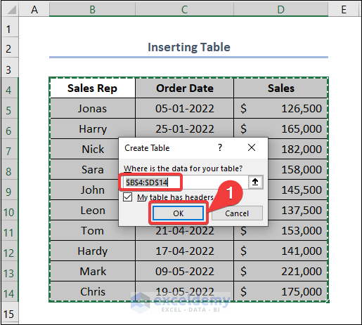
• In the Create Table dialog box, our data range is already selected.Click OK.

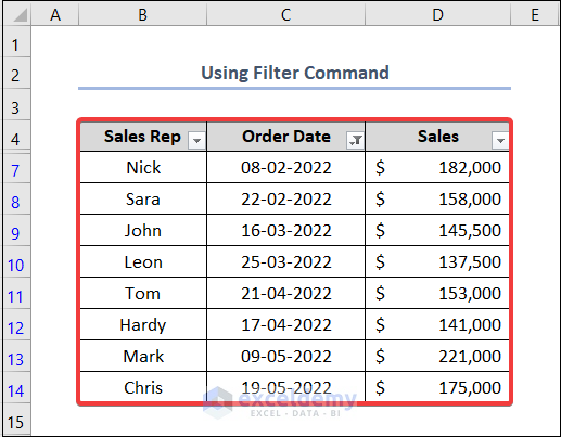
• The Filter Data icon beside each header. You can use this icon to navigate the Date Filters option.

• Click on the Filter icon in the Order Date’s header, and you can filter your data by date easily, just like our previous method.

Method 3 – Create Pivot Table to Group Dates

Steps:

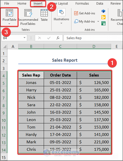
• Create a pivot table select the range of data in our Dataset worksheet. From the Insert tab, select Pivot Table.

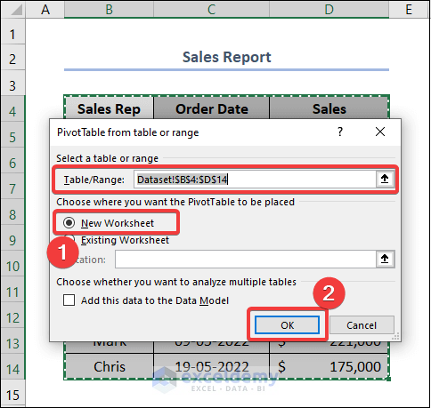
• The PivotTable from table or range dialog box opens. Our dataset is already selected in the table selection box. Choose New Worksheet to place our pivot table, and click OK.

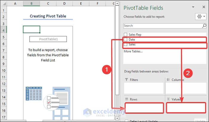
• The new worksheet interface will look like the image below. Drag down 2 fields Date and Sales into Rows and Values.

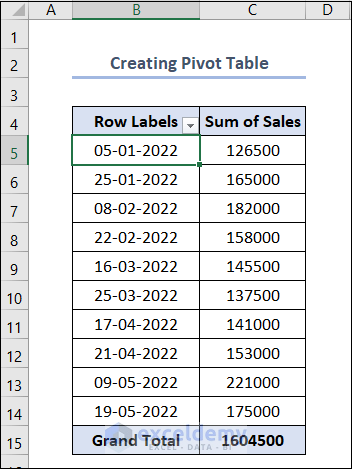
• Our pivot table is looking like this.

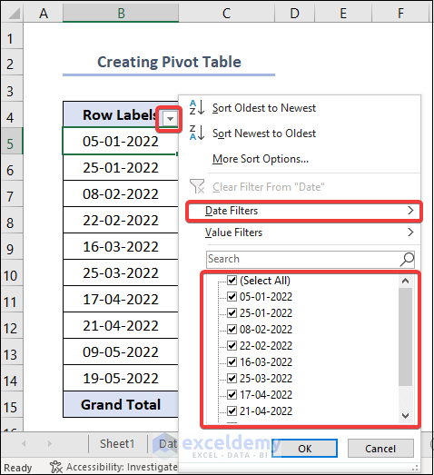
• There is a drop-down arrow beside each header. Click the arrow beside Row Labels’ header to filter data by date like Method 1.

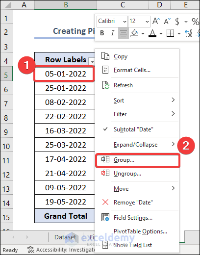
• To group dates, select any date from Row Labels and right-click on it. Choose the Group option from the list.

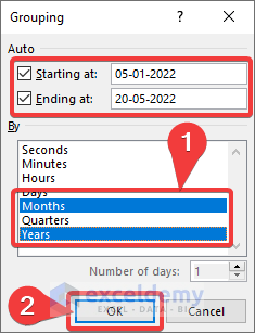
• The Grouping dialog box opens. You can see that starting and ending dates are automatically set. Choose Months and Years from the list to group the data by this condition. Click OK.

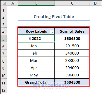
• You can see that our table is magically transformed to show the data in months and years instead of the date format. We can easily visualize the monthly total sales. Here our dates are grouped into months as per our preference.

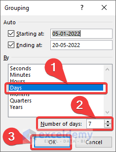
• Group dates on a weekly base. Select Days and write down 7 in the Number of days box in the Grouping dialog box. Click OK.

• Our pivot table shows just like below.

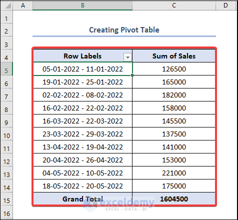
Our Order Dates are now grouped into weeks with a range of 7 days.

Possible Reasons If You’re Unable to Group Dates by Filter in Excel

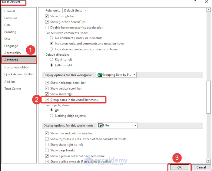
Reason 01: If Grouping Dates in Filters Is Disabled

Solution:

• Select File > Options > Advanced > Check box Group dates in the AutoFilter menu.

Reason 02: When Your Filter Doesn’t Cover All Rows

Solution:

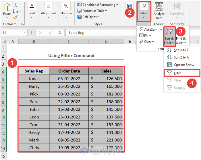
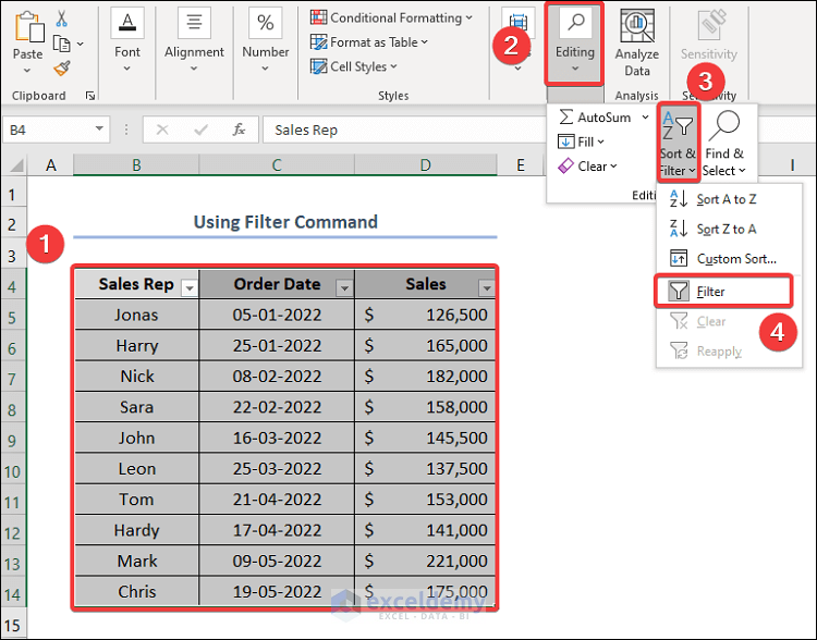
• Select filtered cells on your worksheet. Select as follows.

Editing > Sort & Filter > Filter.

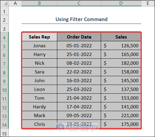
• We filtered range of cells will look like this.

• Add a Filter following Method 1

Download Practice Workbook

You may download the following Excel workbook for better understanding and practice yourself.

<< Go Back to Date Filter | Filter in Excel | Learn Excel