How to Filter Last 30 Days of Date in Excel (5 Easy Ways)

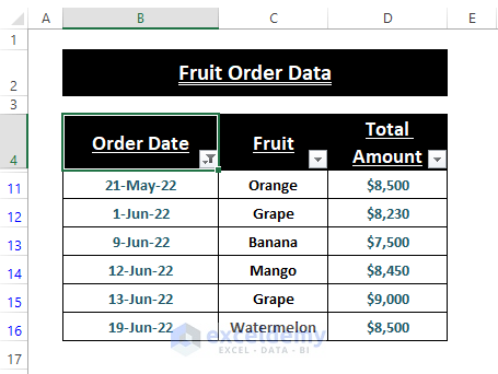
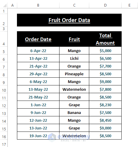
Suppose we have the following dataset containing dates along with other entries, and we want to filter the dataset to only show entries from the last 30 days.

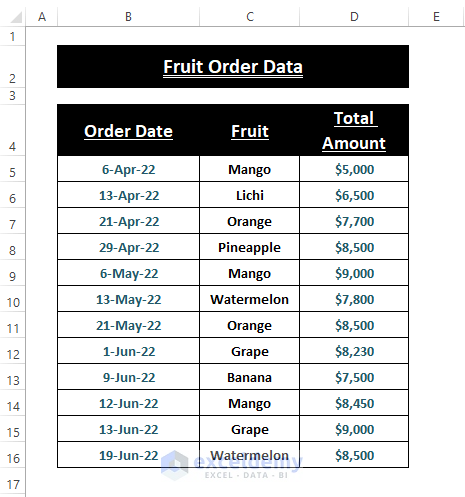
In this article, we’ll demonstrate how to use the Filter feature, VBA Macro, TODAY function, the FILTER function as well as the Power Query to accomplish this task.

Method 1 – Using the Filter Feature

To date-filter a certain number of days, we can use the Filter option Between.

Steps:

• Place your cursor in any cell.
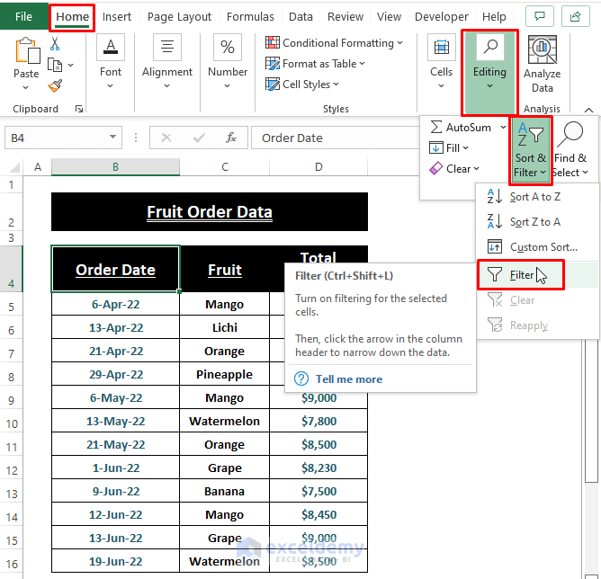
• Go to the Home tab > Editing section.
• Click on Sort & Filter.
• Click on Filter.

Excel enables the Filter feature for the columns.

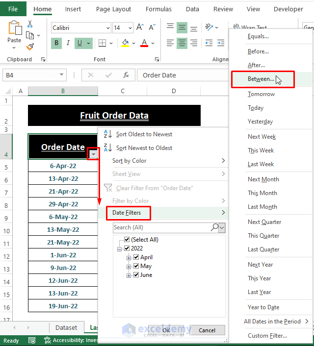
• Click on the Filter Icon.
• Select Date Filters.
• Click on the option Between.

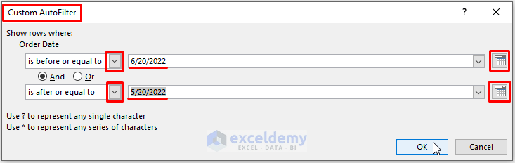
The Custom AutoFilter window opens.

• Under Show rows where, select respective dates for is before or equal to and is after or equal to using the Calendar icons.
• Click OK.

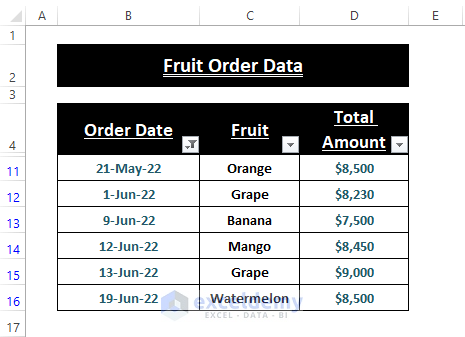
Excel filters the worksheet’s entries to those within the last 30 days.

Similarly, filter the entries for the last 60 or 90 days, or as desired.

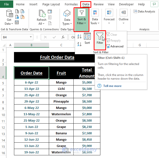
• Alternatively, apply the Filter feature by going to the Data tab > Sort & Filter section > Filter.

Method 2 – Using Excel VBA

VBA Macros allow users to write their own functions, as we will do here with a sub-procedure called FilterToLastNDays.

Steps:

• Press ALT+F11 to open the Microsoft Visual Basic window.
• Alternatively, go to the Developer tab > Visual Basic > Insert > Module.

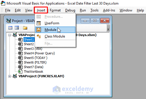
• Copy the following code and paste it in the Module window:

Sub FilterLast30Days()
FilterToLastNDays 30
End Sub
Sub FilterToLastNDays(N As Integer)
With Worksheets("VBA").Range("$B$4")
.AutoFilter
.AutoFilter Field:=1, Criteria1:=">=" & Date - N, Operator:=xlAnd, Criteria2:="<=" & Date
End With
End Sub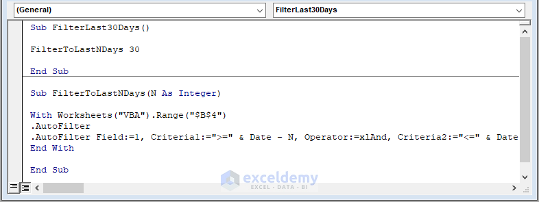

In the code, the first macro holds the FilterToLastNDays function to filter the last 30 days, then the second macro defines the assigned function. The WITH statement provides the worksheet and ranges for filtering. The AutoFilter command assigns the necessary criteria to execute the filtering.

• Press F5 to run the macro.
• Return to the worksheet.

Excel filters the entries according to the given criteria.

Simply edit the number of days after the FilterToLastNDays function to change the filter range.

Method 3 – Using AND and TODAY Functions

The AND function takes multiple logic as its arguments. We’ll insert the TODAY function as an argument to assign dates as criteria.

Steps:

• Add a helper column adjacent to the dataset.
• Copy and paste the following formula in cell E5:

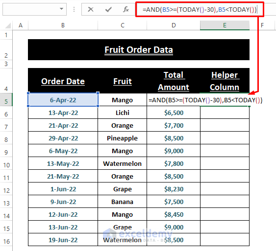
The ADD function takes B5>=(TODAY()-30 as its Logical1 and TODAY() as Logical2 arguments.

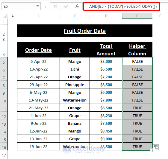
• Press ENTER to return the result.
• Drag the Fill Handle down to display the logical outcomes of TRUE or FALSE in the rest of the column.

• Apply the Filter feature by following the first Step of Method 1.
• Click on the Filter Icon.
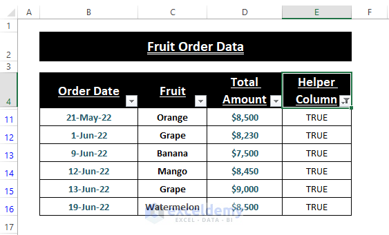
• Mark only the TRUE option.
• Click on OK.

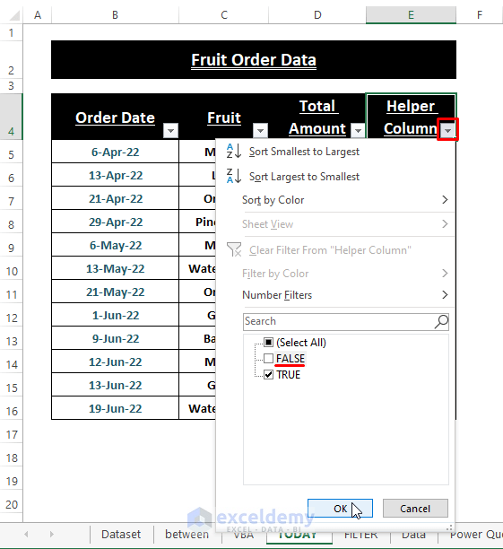
Excel displays only the entries within the last 30 days.

Method 4 – Using the FILTER Function

The FILTER function is only available in the Excel 365 version.

The syntax of the FILTER function is:

FILTER (array, include, [if_empty])

Steps:

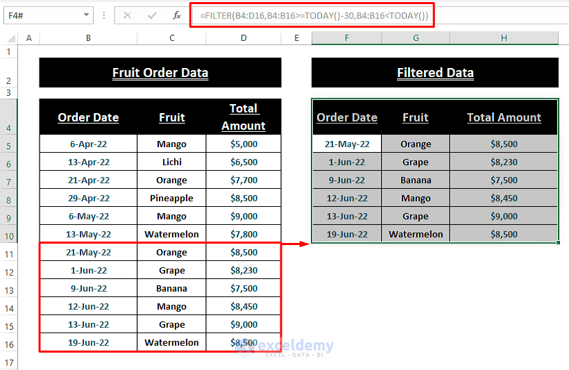
• Enter the following formula in cell F4:

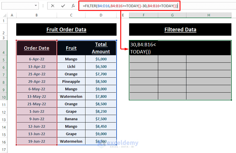
In the formula, B4:D16 is the array, B4:B16>=TODAY()-30 is the function to include and B4:B16<TODAY() is the function to run [if_empty].

• Press ENTER to fetch all the entries that match the criteria.

Method 5 – Using Power Query

The in-built Power Query tool also offers a Filter Feature.

Steps:

• Highlight the range.
• Go to the Data tab.
• Click on From Table/Range (under Get & Transform Data).

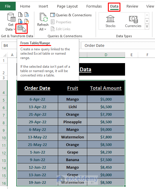
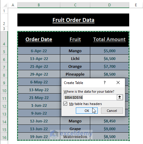
Excel opens a Create Table window and automatically sets the range.

• Tick the My table has headers option.
• Click on OK.

Excel loads the data.

• Click on the Filter Icon of the Order Date column.
• Click on Date/Time Filters > Between.

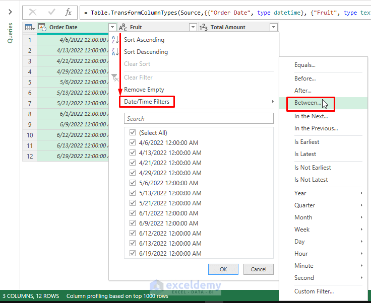
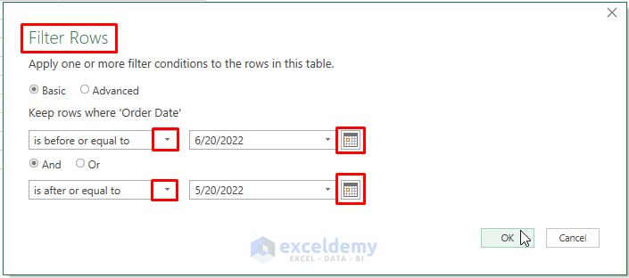
Excel opens the Filter Rows dialog box.

• Choose And logic.
• Provide dates to encompass 30 or the desired number of days.
• Click on OK.

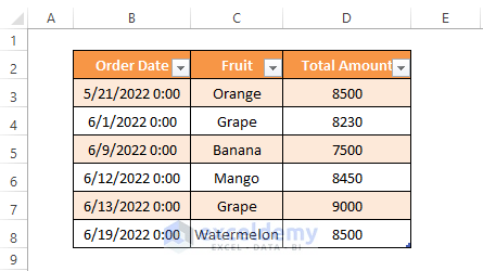
Excel loads the filtered data.

• Click Close & Load.
• Click Close & Load again.

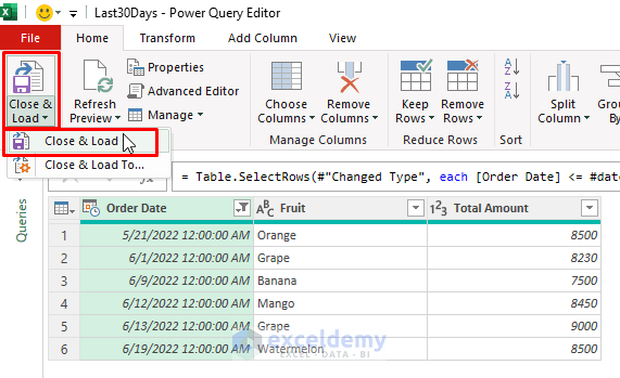
The filtered data are loaded into a new worksheet.

Download Excel Workbook

<< Go Back to Date Filter | Filter in Excel | Learn Excel