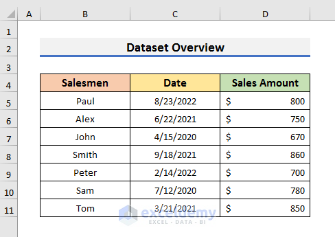
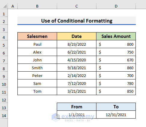
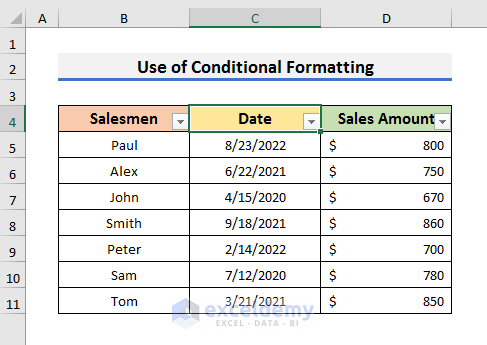
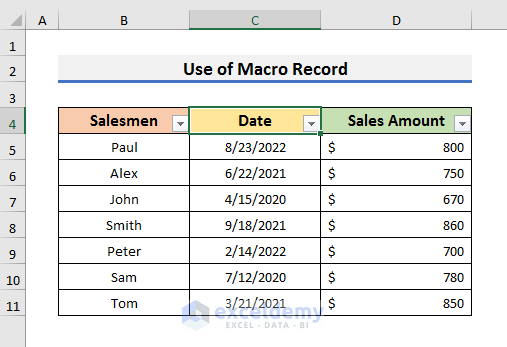
We will use a dataset that contains information about the Sales Amount on different dates for some salesmen. We will use the custom date filter in the dataset and show the sales amount for specific dates. The same dataset will be used throughout the whole article.
Method 1 – Use the Filter Command to Apply a Custom Date Filter in Excel
STEPS:
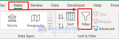
- Select a cell in your dataset.
- Go to the Data tab and select Filter.
- A drop-down arrow will appear in the headers of the dataset.
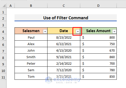
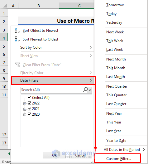
- Click on the drop-down arrow to open the Context Menu.
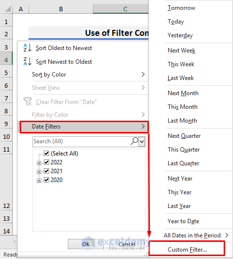
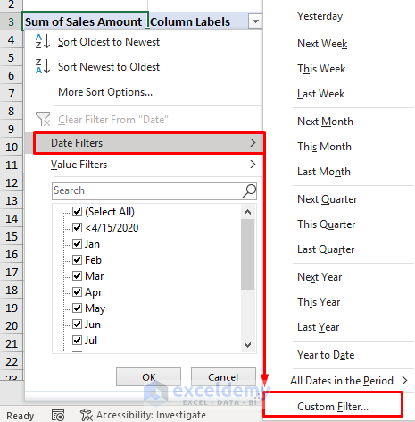
- From the Context Menu, select Date Filters and then select Custom Filter.
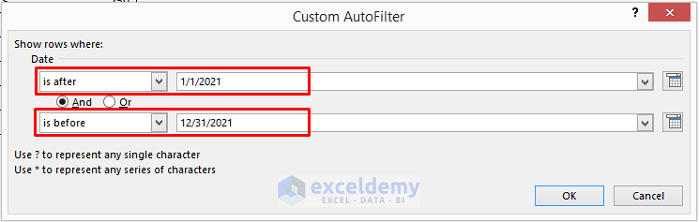
- The Custom AutoFilter window will appear.
- Select ‘is after’ and type ‘1/1/2021’ in the first field.
- In the second field, select ‘is before’ and type ‘12/31/2021’.
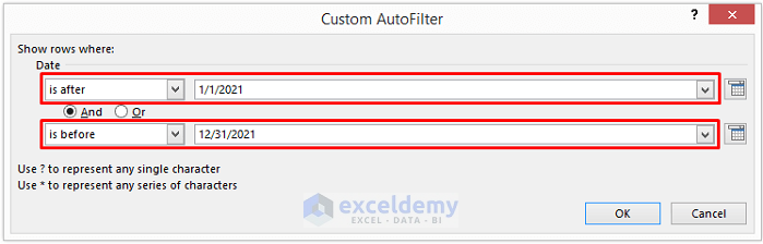
We want to filter the sales amount from 1/1/2021 to 12/31/2021. You can change this section according to your needs.
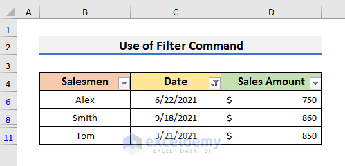
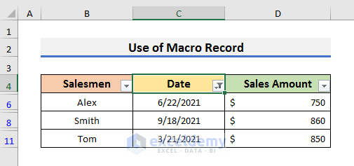
- Click OK to see results like the picture below.
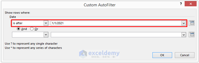
- If you want to filter the sales amount after 1/1/2021, you can select ‘is after’ and type ‘1/1/2021’ in the first field only.
- Click OK to proceed.
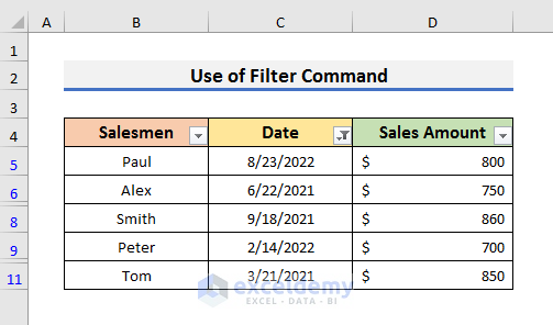
- You will see this result.
Method 2 – Apply a Custom Date Filter Using Excel Conditional Formatting
STEPS:
- Type the Starting Date and Ending Date outside of the main dataset. We want to filter the values from 1/1/2021 to 12/31/2021. We put 1/1/2021 and 12/31/2021 in cells C14 and D14, respectively.
- Select Cell F5 and insert this formula:
=AND(C5>=$C$14,C5<=$D$14)- Hit Enter to see the result.
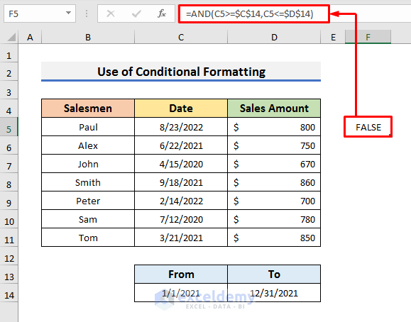
We have used the AND function. This formula checks if the value of Cell C5 is between 1/1/2021 and 12/31/2021. If it is between 1/1/2021 and 12/31/2021, then, it will show TRUE. Otherwise, it will display FALSE.
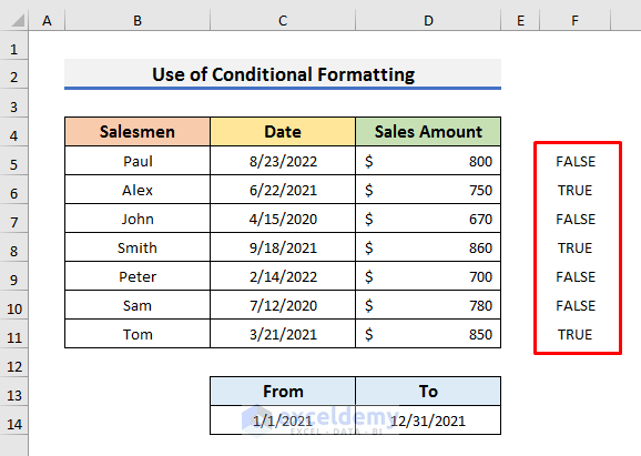
- Drag the Fill Handle down.
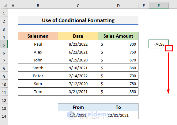
- You can see the results in the picture below.
- Select Cell C4 and press Ctrl + Shift + L to apply a Filter in the dataset. You can also do this from the Data tab like Method 1.
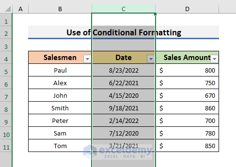
- Select Column C.
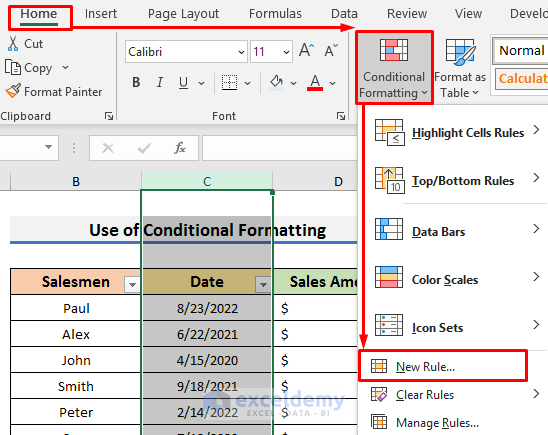
- Go to the Home tab and select Conditional Formatting.
- Select New Rule to open the New Formatting Rule window.
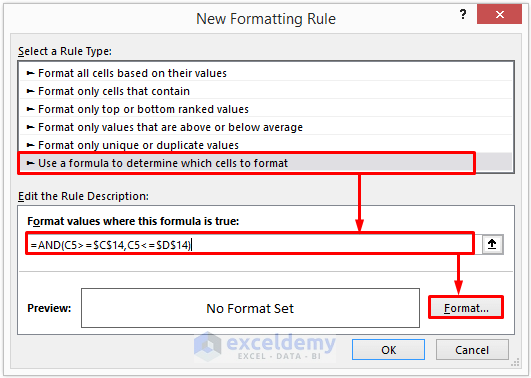
- Select ‘Use a formula to determine which cells to format’.
- Insert the formula:
=AND(C5>=$C$14,C5<=$D$14)- Select Format.
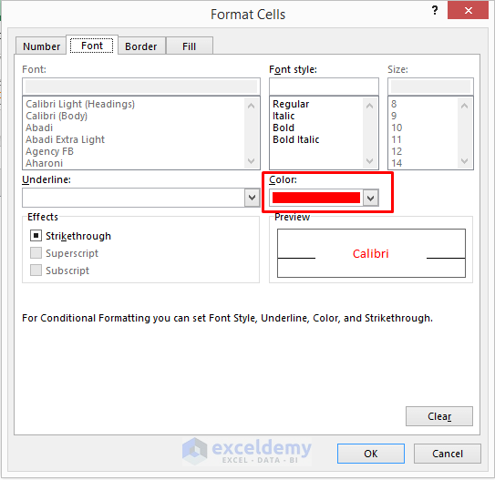
- Change the Font Color to Red and click OK to proceed.
- Click on the drop-down arrow in the Date column.
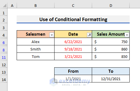
- Select Filter by Color and then select the Red color.
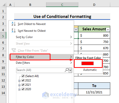
- You will see results like the picture below.
Method 3 – Use a Custom Date Filter with a Pivot Table
STEPS:
- Select a cell in the dataset.
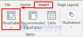
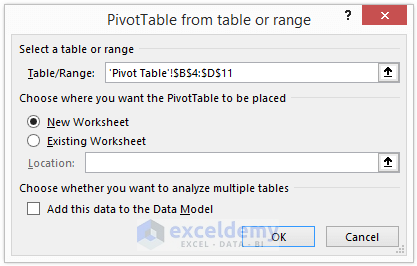
- Navigate to the Insert tab and select the PivotTable icon.
- A message will pop up.
- Click OK to proceed.
- A new sheet will open with the PivotTable Fields on the right panel.
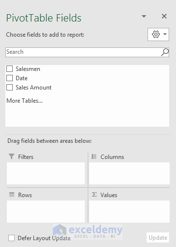
- Drag Salesmen, Date, and Sales Amount in the respective PivotTable Fields section.
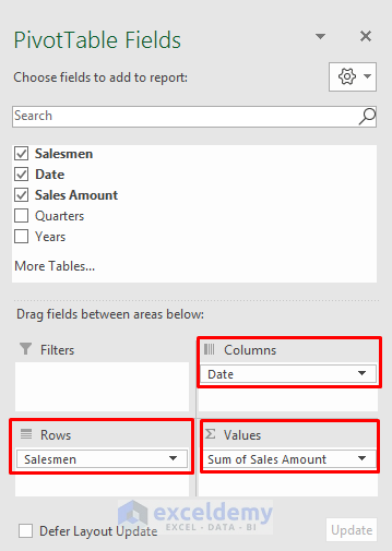
- Click on the drop-down arrow of the Column Labels column.
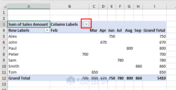
- From the drop-down menu, select Date Filters and then select Custom Filter. It will open the Date Filter (Date) window.
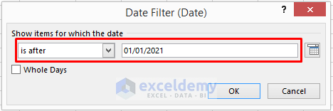
- Select ‘is after’ and type 01/01/2021. It denotes that the pivot table will contain values from the date 01/01/2021.
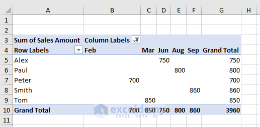
- You will see the filtered results like the picture below.
Method 4 – Insert a Formula to Use a Custom Date Filter in Excel
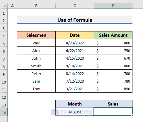
We will use a formula to filter the Sales Amount for August. The formula will look for the sales for August irrespective of the year. We have added a section for the Month and the Sales amount.
STEPS:
- Select Cell D14.
- Insert the formula below:
=FILTER(D5:D11,MONTH(C5:C11)=8,"Empty")- Press Enter to see the results.
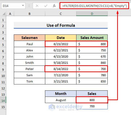
- The first argument (D5:D11) is the array where it looks for the Sales Amount.
- The second argument MONTH(C5:C11)=8 denotes that the month is August.
- If it finds no value of August, then it prints Empty.
Method 5 – Use Excel Macro Record to Apply a Custom Date Filter
STEPS:
- Select a cell in the dataset and press Ctrl + Shift + L to apply a Filter.
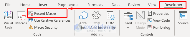
- Go to the Developer tab and select Record Macro. It will open the Record Macro window.
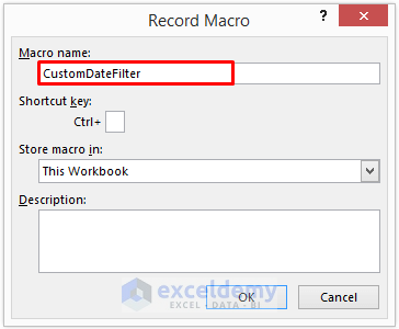
- In the Record Macro window, type a name for the macro and click OK to proceed. We have named it CustomDateFilter.
- Click on the drop-down arrow in the Date column.
- Select Date Filters and then select Custom Filter. It will open the Custom AutoFilter window.
- In the Custom AutoFilter window, select ‘is after’ and type ‘1/1/2021’ in the first field.
- In the second field, select ‘is before’ and type ‘12/31/2021’.
- Click OK to proceed.
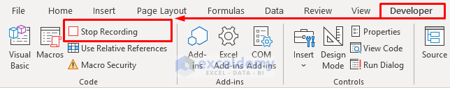
- Navigate to the Developer tab and select Stop Recording.
- Open a similar sheet where you have the same dataset.
- Go to the Developer tab and select Macros from there.
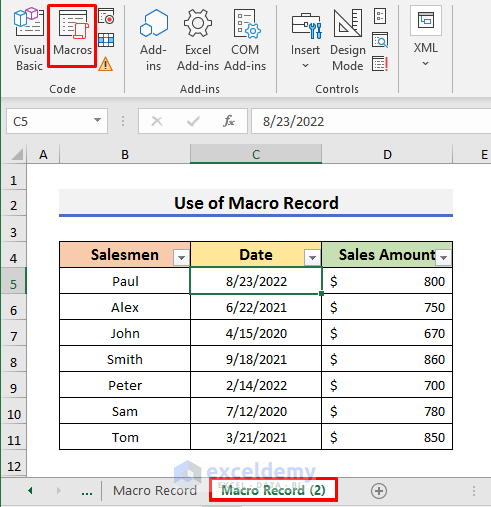
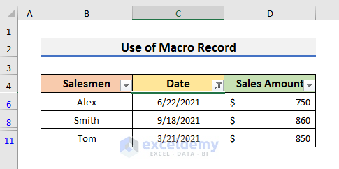
- Click on Run in the Macro window.

- You will get the results like the picture below.
Download the Practice Book
<< Go Back to Date Filter | Filter in Excel | Learn Excel
Get FREE Advanced Excel Exercises with Solutions!

Hi! can you filter dates older than a set number of days from today? I tried the is before Today-35 bit that didn’t work
Hi SEM,
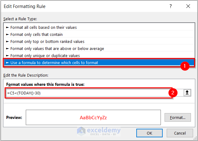
Thanks for your comment. I am replying to you on behalf of ExcelDemy. If you want to filter dates older than a number of days from today, you can follow the steps from Method-2. But, instead of the formula used here, write the following formula.
=C5<(TODAY()-30)Here, I wrote the formula for dates older than 30 days from today. You can change the formula according to your preference.
I hope this will help you to solve your problem. Please let me know if you have other queries.
Regards
Mashhura
ExcelDemy