How to Create a Color Scale with Conditional Formatting Based on Another Cell

Dataset Overview

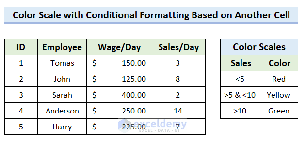
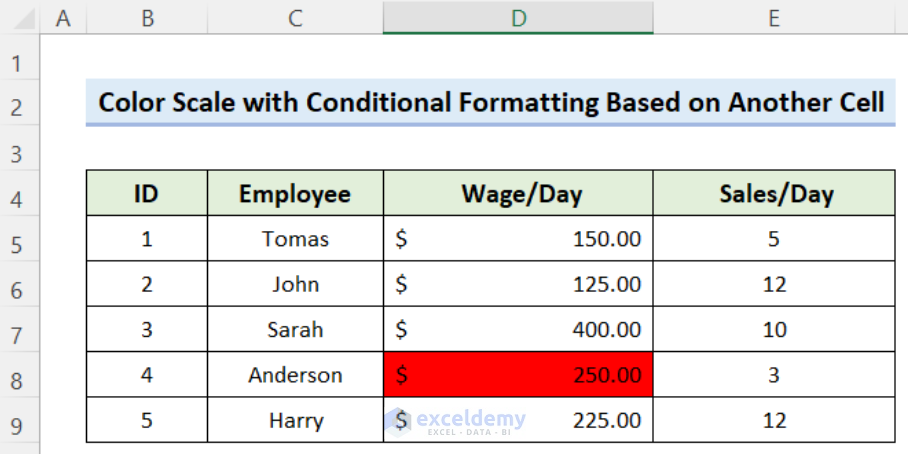
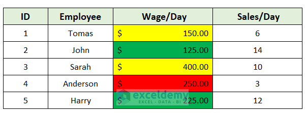
Suppose you have a dataset with daily wages and sales data. You want to format the wages column using a color scale based on the sales value. Here’s how you can do it:

Step 1 – Define the Conditions

• Select the Wages Column:
  • Highlight the cells in the Wages/Day column where you want to apply the color scale.
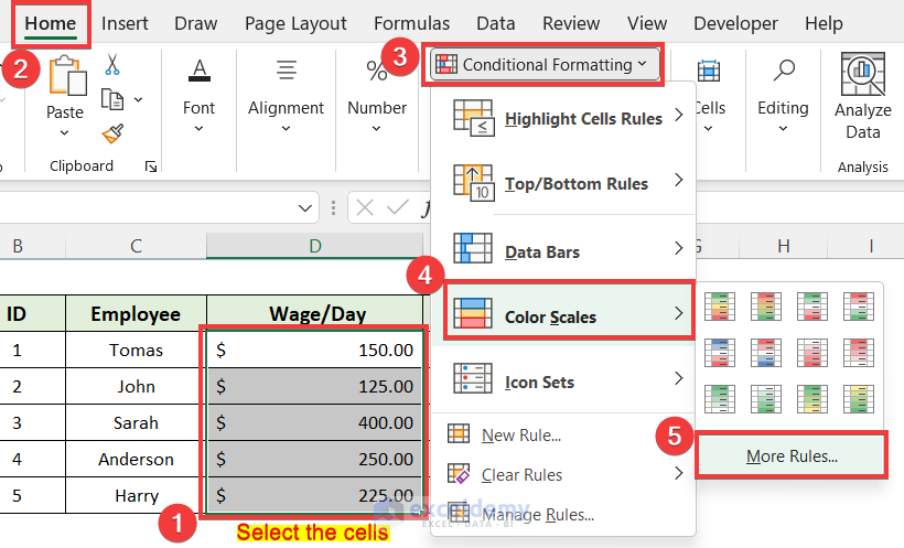
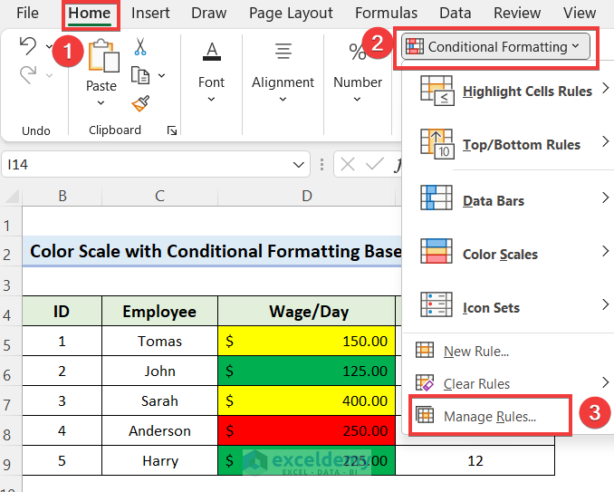
• Access Conditional Formatting:
  • Go to the Home tab in the Excel ribbon.
  • Click on Conditional Formatting and choose Color Scales.
  • Then select More Rules.

Step 2 – Set Up Formulas and Colors for Different Conditions

We’ll create three rules corresponding to different sales value ranges:

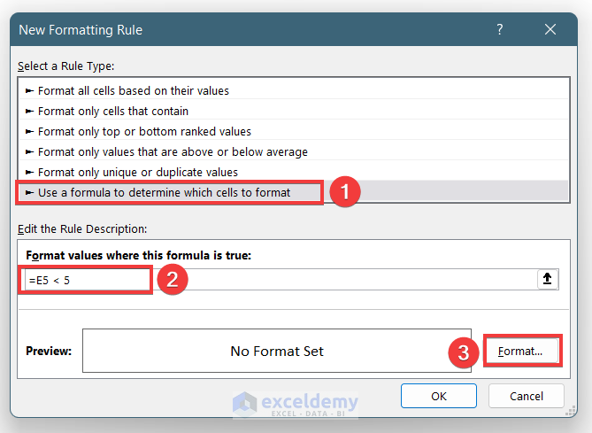
• Red for Sales < 5:
  • In the New Formatting Rule window, choose Use a formula to determine which cells to format.

• • Enter this formula in the rule box:

• • Click Format.

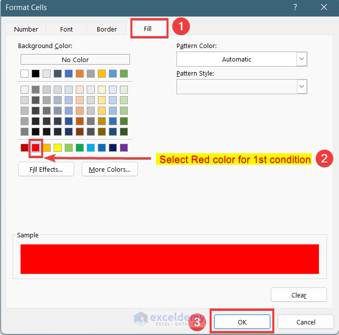
• • Go to the Fill tab and select the Red as Background Color.
  • Press OK.

• • The wage cell has become red if sales/day is less than 5.

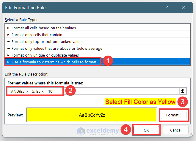
• Yellow for Sales Between 5 and 10:
  • Create a similar rule:

• • Enter this formula into the rule description box

• • Format with yellow background.

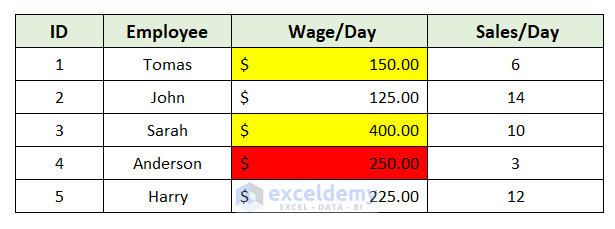
• • The cells of wages become yellow of which sales/day is between 5 and 10.

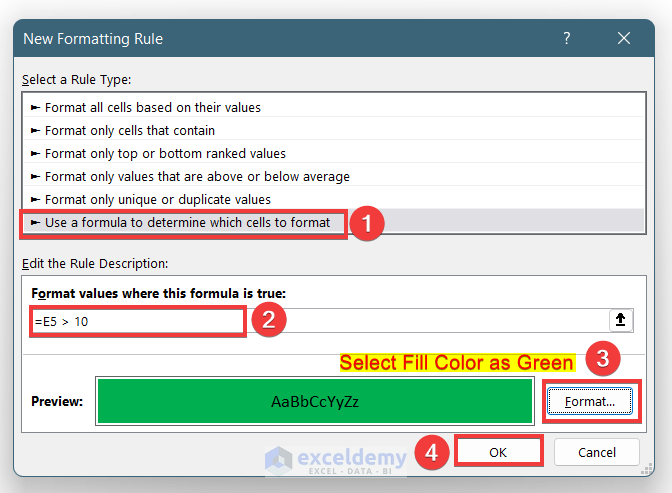
• Green for Sales > 10:
  • Again, create a rule:

• • Enter this formula in the box:

• • Format with green background.

• • The cells of wage/day of rows where sales/day is greater than 10 become green.

Read More: Conditional Formatting with 3 Color Scale in Excel Formula

Step 3 – Organize the Rules

To ensure the rules are applied in the correct order:

• Go to the Home tab.
• Click on Conditional Formatting and select Manage Rules.

• In the Stop If True column, check all the boxes.

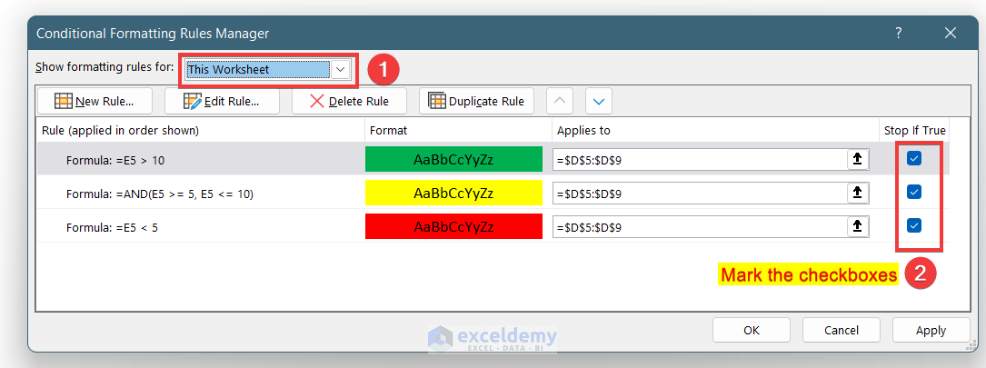
• Arrange the rules:
  • Drag the rule for Sales < 5 to the top.
  • Place the rule for Sales between 5 and 10 next.
  • The rule for Sales > 10 will be automatically positioned last.

• Now, when you change the values in the Sales column, the color of the wage cells will adjust accordingly.

Read More: Color Scale Per Row with Conditional Formatting in Excel

Things to Remember

• Directly applying color scale formatting based on another cell isn’t possible in Excel.
• You need to create individual rules for each condition to achieve the desired color scale effect.

Download Practice Workbook

You can download the practice workbook from here:

Related Articles

• How to Use 4 Color Scale Conditional Formatting in Excel
• How to Use Conditional Formatting with 5 Color Scale in Excel
• How to Use Excel Color Scale Based on Text

<< Go Back to Conditional Formatting | Learn Excel