How to Use Conditional Formatting with 5 Color Scale in Excel (2 Methods)

We have financial information about some wrestling superstars: their Yearly Income and Net Worth. We’ll format the data in a five-color-scale.

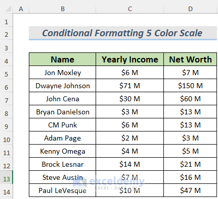
excel conditional formatting 5 color scale

Method 1 – Using the Built-In Command to Apply Conditional Formatting with a 5-Color Scale

Steps:

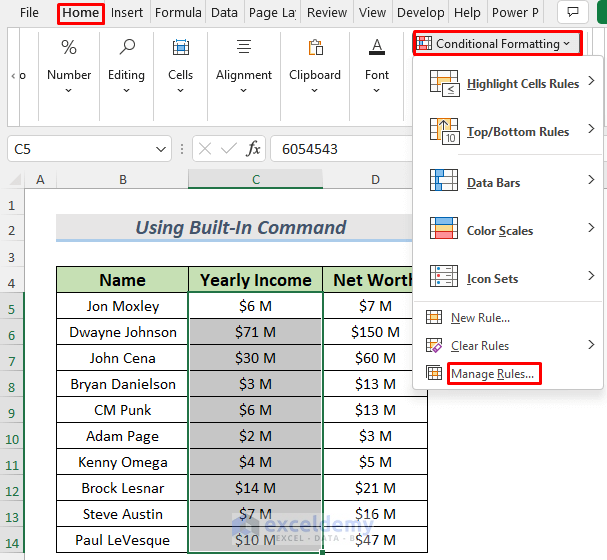
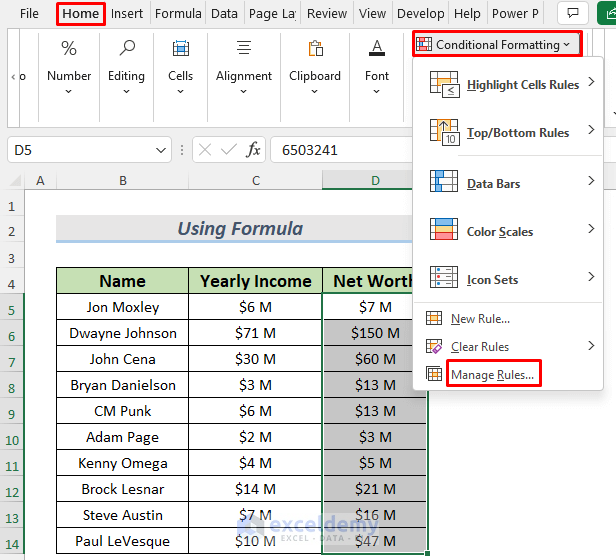
Select a column and go to Conditional Formatting.
Select Manage Rule.

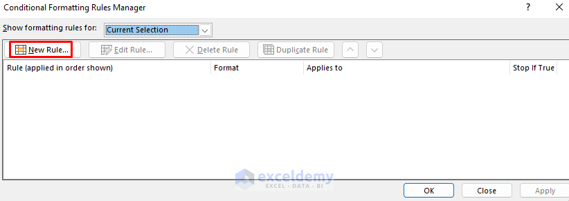
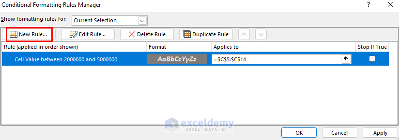
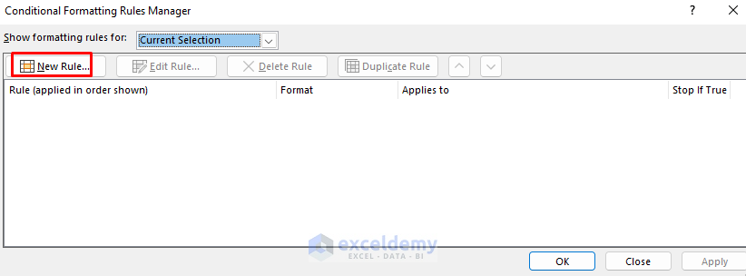
You will see the Conditional Formatting Rules Manager.
Select New Rule (you can also use that option directly from the Conditional Formatting drop-down in the ribbon).

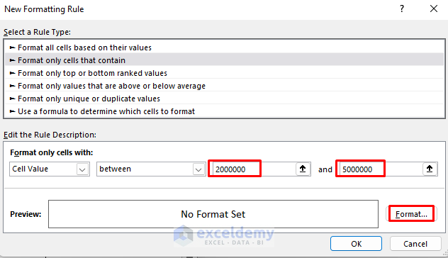
excel conditional formatting 5 color scale

The New Formatting Rule window will open.
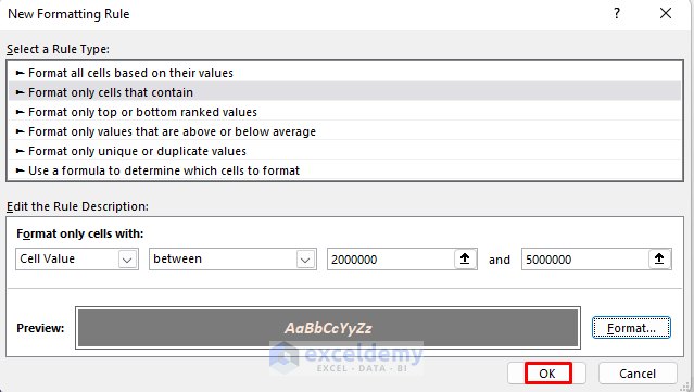
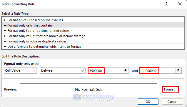
Select any Rule Type of your choice. We chose Format only cells that contain.
Set a range in the Edit the Rule Description section.
Select Format…

Select Fill and choose any color.

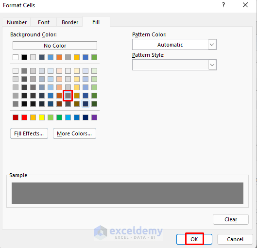
excel conditional formatting 5 color scale

Select a Font and a suitable Font Color. If you want to fill the cell background with a darker color, select a lighter font color.
You can also select other options like Font Style or effects. In this case, we just selected Bold Italic.
Click OK.

The New Formatting Rule window will appear again. Click OK.

excel conditional formatting 5 color scale

You will see that the rule has been added to the Conditional Formatting Rules Manager. This will format the cells that contain this range of values.
To set another rule, click on New Rule…

Set a new range like before.

excel conditional formatting 5 color scale

Repeat to make five rules to format the cells for a five-color-scale conditional formatting section. Each rule uses a different background color from the Fill tab and the appropriate font options to make the text visible.
Click OK.

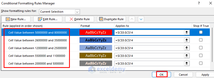
You will see the data formatted to a 5-color-scale.

excel conditional formatting 5 color scale

Method 2 – Applying a Formula to Utilize Conditional Formatting with a 5-Color Scale

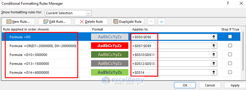
In this section, we’ll format the Net Worth values. We’re showing you the rules we created. There are five different formulas for the 5-color-scale conditional formatting.

Steps:

Select the Net Worth values and then go to Conditional Formatting and select Manage Rules.

excel conditional formatting 5 color scale

Select New Rule… from the Conditional Formatting Rules Manager window.

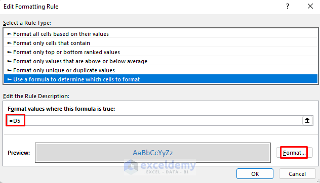
Choose Use a formula to determine which cells to format and insert the following formula in it.

=D5

Select Format…

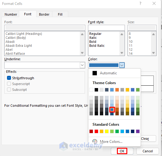
excel conditional formatting 5 color scale

In the Format Cells window, select a font color of your choice.

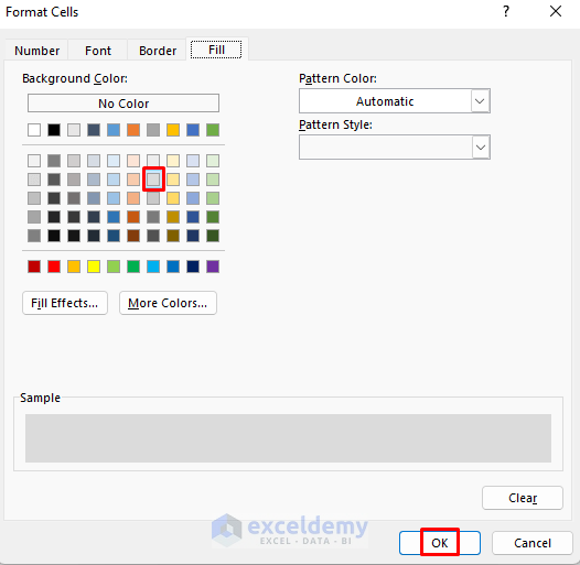
Select a Fill color and click OK.

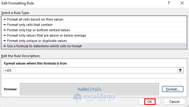
excel conditional formatting 5 color scale

The Edit Formatting Rule will appear again. Click OK.

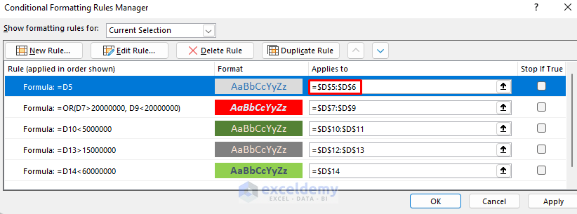
The formula will be added to the Rules Manager as the number one rule. You can edit the range for the rules after that.
We added four other formulas and ranges that you can see in the following image one by one. You may apply your own formulas or functions. In the second rule, we used the OR function.
Click OK.

excel conditional formatting 5 color scale