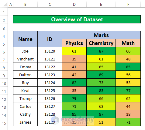
The sample dataset is a large Excel worksheet containing information about several students.
Method 1 – Using the IF Function to Apply Conditional Formatting with a 3 Color Scale
Step 1:
- Select D6:F15.
- In the Home tab, go to
Home → styles → Conditional Formatting → Manage Rule

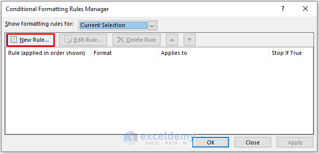
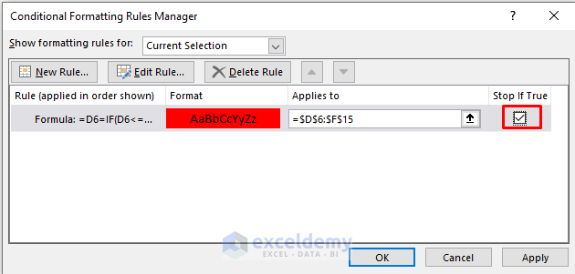
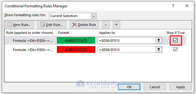
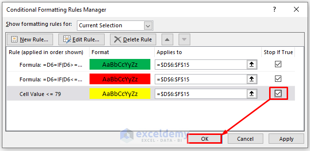
- The Conditional Formatting Rules Manager dialog box opens.
- Click New Rule.
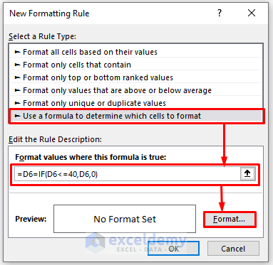
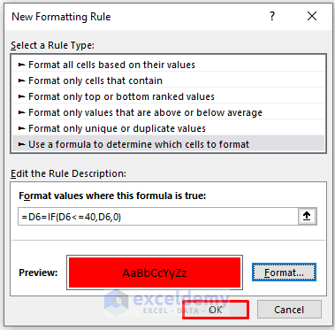
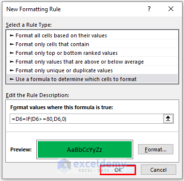
- In the New Formatting Rule dialog box, select Use a formula to determine which cells to format.
- Enter the following formula :
=D6=IF(D6<=40,D6,0)- It will highlight cells whose value is less than or equal to 40.
- Click Format.
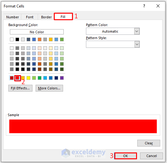
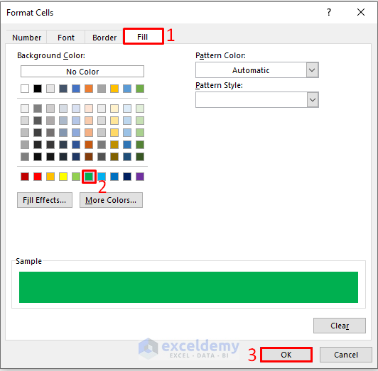
- In the Format Cells dialog box, select Fill.
- Choose a color, here Red.
- Click OK.
- Click OK.
- Check Stop IF True (to make sure your formula will work for rows only)
- Click New Rule to add more formulas.
Step 2:
- Click New Rule.
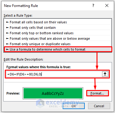
- In the New Formatting Rule dialog box, select Use a formula to determine which cells to format.
- Enter the following formula :
=D6=IF(D6>=80,D6,0)- It will highlight the cells whose value is greater than or equal to 80.
- Click Format.
- In the Format Cells dialog box, select Fill
- Choose a color, here Green.
- Click OK.
- Click OK.
- Check Stop IF True (to make sure your formula will work for rows only).
- Click New Rule to add more formulas.
Step 3:
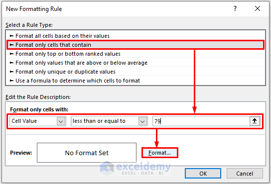
- Click New Rule. The New Formatting Rule dialog box will open
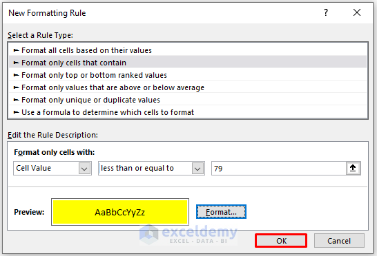
- In the New Formatting Rule dialog box, select Format only cells that contain.
- Select Cell Value.
- Choose less than or equal to.
- Enter 79 under Format only cells with.
- Click Format.
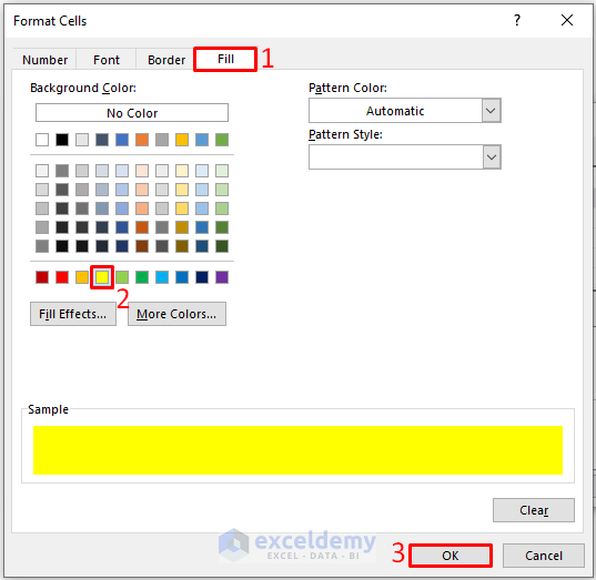
- In the Format Cells dialog box, select Fill.
- Choose a color, here Yellow.
- Click OK.
- Click OK.
- Check Stop IF True (to make sure your formula will work for rows only)
- Click New Rule to add more formulas.
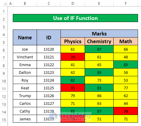
This is the output.
Read More: How to Use 4 Color Scale Conditional Formatting in Excel
Method 2 – Applying a 3 Color Scale Command in Conditional Formatting
Step 1:
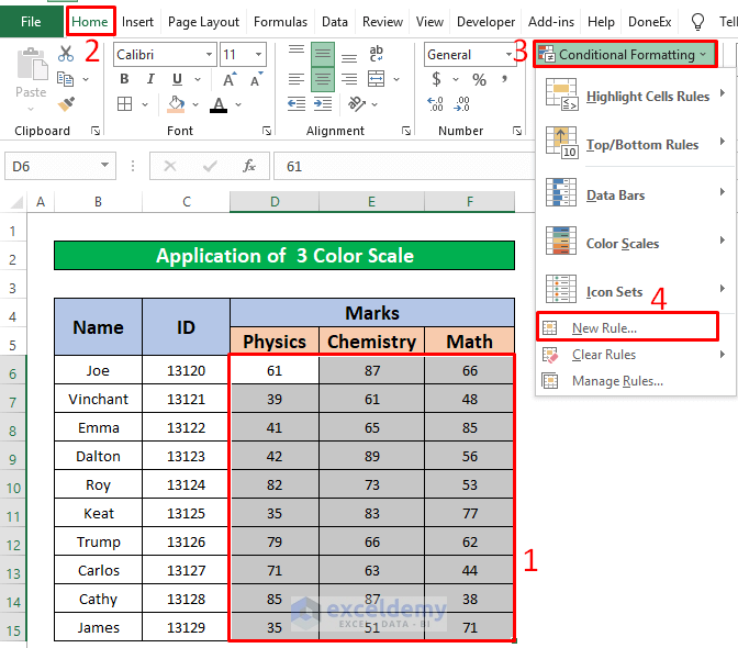
- Select D6:F15.
- In the Home tab, go to
Home → styles → Conditional Formatting → New Rule
Step 2:
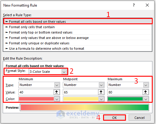
- Click New Rule to see the New Formatting Rule dialog box.
- In Select a Rule Type, select Format all cells based on their values.
- In Format Style, select 3-Color Scale.
- In Minimum, select Number from the Type drop-down list. Enter 40 in Value. Select Orange from the Color drop-down list.
- In Midpoint, select Number from the Type drop-down list. Enter 65 in Value. Select Yellow from the Color drop-down list.
- In Maximum, select Number from the Type drop-down list. Enter 80 in Value. Select Green from the Color drop-down list.
- Click OK.
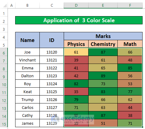
This is the output.
Read More: Color Scale Per Row with Conditional Formatting in Excel
Things to Remember
- You also can use the AND function instead of the IF function in conditional formatting with 3-color scale. The AND function is,
For Red color: =AND(D6<40)
Yellow: =AND((D6>=40),(D6<80))
Green: =AND(D6>=80)
- #N/A! error arises when the formula or a function in the formula fails to find the referenced data.
- #DIV/0! error is displayed when a value is divided by zero(0) or the cell reference is blank.
Download Practice Workbook
Download this practice workbook to exercise.
Related Articles
- Excel Conditional Formatting Color Scale Based on Another Cell
- How to Use Excel Color Scale Based on Text
- How to Use Conditional Formatting with 5 Color Scale in Excel
<< Go Back to Conditional Formatting | Learn Excel
Get FREE Advanced Excel Exercises with Solutions!
