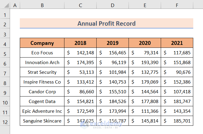
Dataset Overview
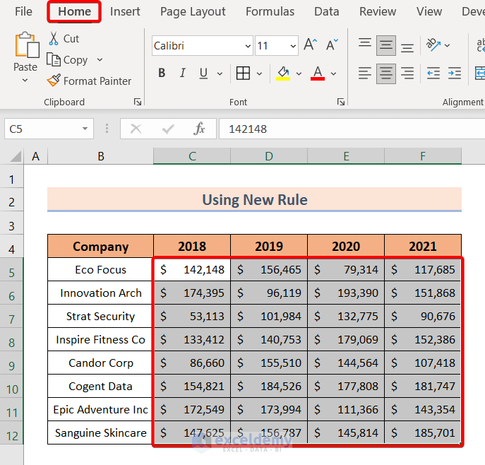
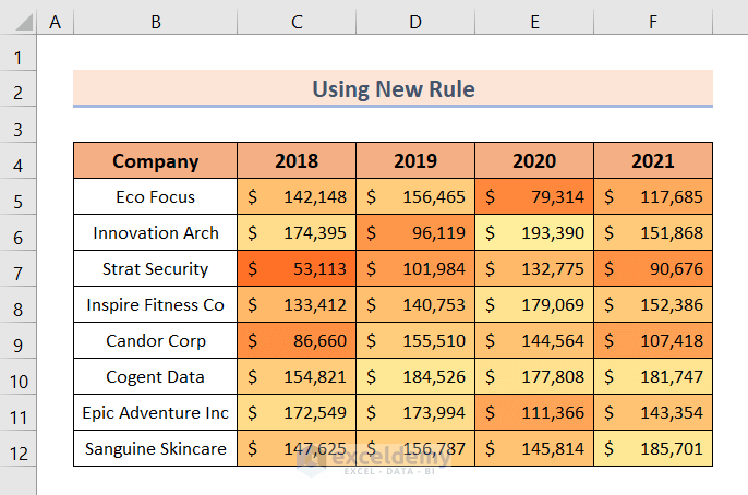
We’ll use the following Annual Profit Record for various companies to demonstrate these methods. In the Company column, there is a list of a few companies. The following columns have their corresponding annual profit records.
Method 1 – Using Conditional Formatting Color Scale Command
- Choose the dataset containing numerical values.
- Go to the Home tab in Excel.
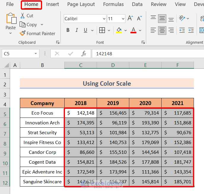
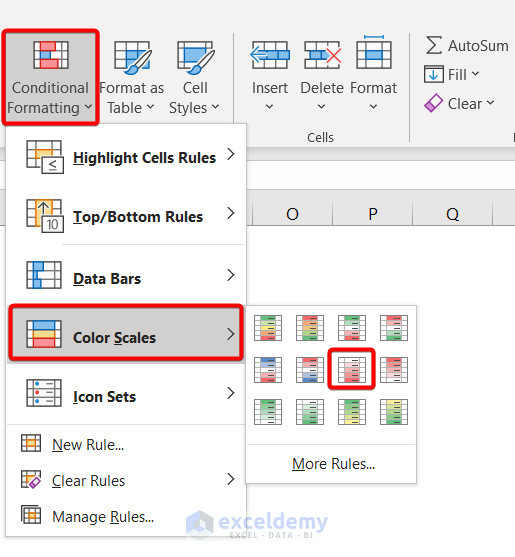
- In the Styles group, click on the Conditional Formatting drop-down.
- From the drop-down list, select Color Scales.
You’ll see various color palettes. Pick one (e.g., White-Red Color Scale).
- Observe your dataset: the minimum value is highlighted in white, and the maximum value in red.
- All values in between are displayed with a gradient of red and white.
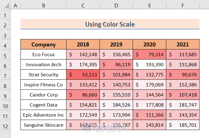
Note: If you apply a color scale to the entire range, Excel uses one global minimum and maximum for the whole dataset. That’s why the darkest and brightest colors only appear on the overall lowest and highest values (e.g., E6 vs. E7).
To apply color scaling per row, you need to set up a separate rule for each row (or use Format Painter to copy a row rule). This way, Excel calculates min–max values within each row, and the highest values in every row will share the same color intensity.
Read More: Excel Conditional Formatting Color Scale Based on Another Cell
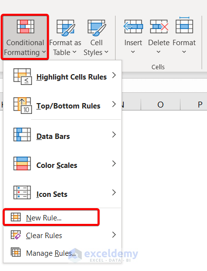
Method 2 – Using New Rule for Conditional Formatting Color Scale Per Row
- Select the dataset with numerical values.
- Navigate to the Home tab.
- Click the Conditional Formatting drop-down in the Styles group.
- Select New Rule.
- In the New Formatting Rule dialog box:
- Choose Format all cells based on their values.
- Select 2-Color Scale as the format style.
- Lowest and highest values are preselected.
- Customize colors if desired (e.g., orange for minimum, gold for maximum).
- Click OK to apply the new rule.
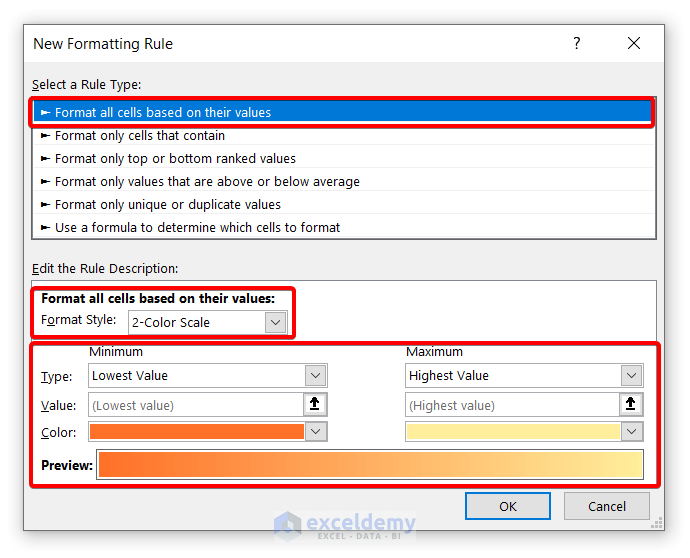
- The minimum value will be highlighted in orange, the maximum in gold.
- Intermediate values will display a gradient between these colors.
Read More: Conditional Formatting with 3 Color Scale in Excel Formula
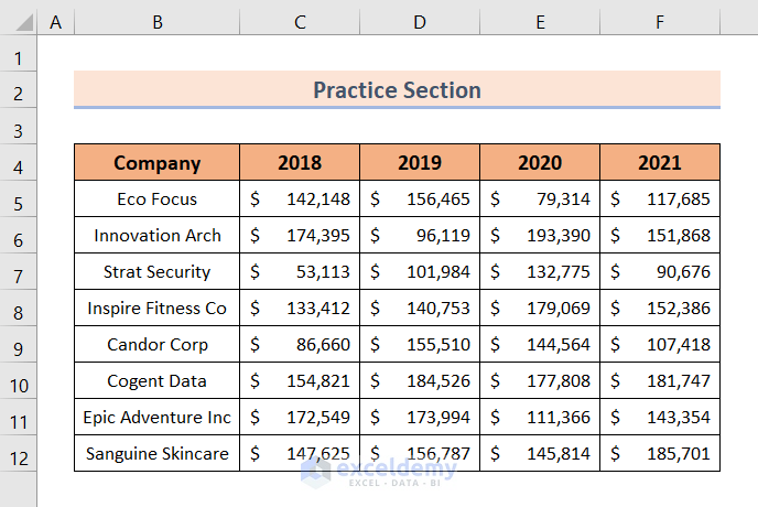
Practice Section
You will get an Excel sheet like the following screenshot, at the end of the provided Excel file where you can practice all the topics discussed in this tutorial.
Download Practice Workbook
You can download the practice workbook from here:
Related Articles
- How to Use Excel Color Scale Based on Text
- How to Use 4 Color Scale Conditional Formatting in Excel
- How to Use Conditional Formatting with 5 Color Scale in Excel
<< Go Back to Conditional Formatting | Learn Excel
Get FREE Advanced Excel Exercises with Solutions!

how do you set the conditional formatting for the set, but the scale is individualized for each row (not all rows data combined)?
As the scale is different for each row, you can apply conditional formatting separately on each row with different colors. I hope that’s the simplest way to do so.
This does not appear to be color scaling by row at all. This is color scaling by the entire range.
Observe E6 and E7. Both are the highest values in their row, and if the color scale were applied by row, they would be the same color.
E7 is a darker color, because it is not color scaling by row. E6 is the highest value in the table, thus it is the only value that has a fully gold color.
Any row with only higher values would show mostly gold colors with no orange values. Any row showing only lower values will have only darker orange values, with no gold.
Hello Eric Esh,
You’re absolutely right—thanks for catching that. In the screenshot the color scale was applied to the entire range, so Excel used one global min→max for the whole table.
That’s why E6 (the overall max) is fully gold while E7 (a row max but not the global max) appears darker.
To truly color-scale by row, each row needs its own color-scale rule.
The quickest way is: Select the first row’s data cells, apply a 3-color scale (Min = Lowest, Mid = 50th percentile or Average, Max = Highest), then use the Format Painter to copy that formatting down to each subsequent row—Excel creates a separate rule per row, so the min/mid/max are computed within that row only.
After doing this, the highest value in every row (like E6 and E7 in your example) will share the same top color, and each row’s gradient will be independent. We mentioned it in the article to make this distinction and the per-row steps clearer—appreciate the sharp feedback.
Regards,
ExcelDemy