How to Use 4 Color Scale Conditional Formatting in Excel (2 Examples)

Excel’s default conditional formatting only goes up to a 3-color scale, so more colors need to be implemented manually.

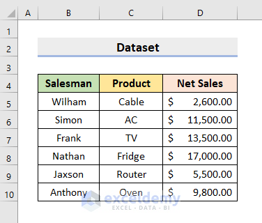
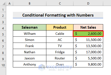
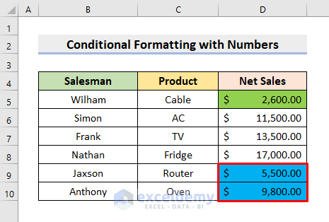
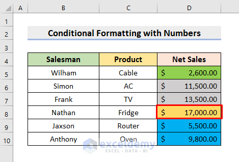
We’ll use a sample dataset as an example. We have Salesman, Product, and Net Sales. We’ll apply the 4-color scale Conditional Formatting to the Net Sales column. We’ll use four criteria for that purpose:

• less than 5,000
• between 5,000 and 10,000
• between 10,000 and 15,000
• more than 15,000

Method 1 – Use a 4-Color Scale Conditional Formatting with Numbers in Excel

STEPS:

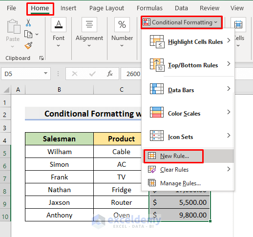
• Select the range D5:D10.

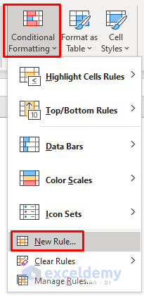
• Under the Home tab, click the Conditional Formatting drop-down icon.
• Choose New Rule.

• A dialog box will pop out.
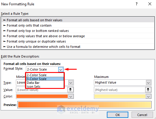
• Click the Format Style drop-down.
• You’ll see that the 2-Color Scale and 3-Color Scale are present. You won’t get the 4-Color Scale.

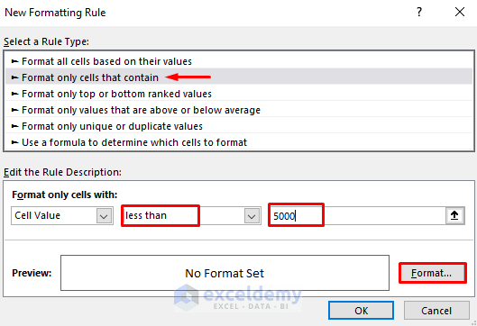
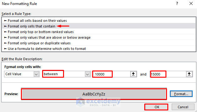
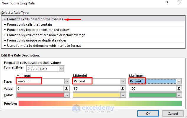
• Select the second Rule Type.
• Choose less than from the second drop-down under the Edit the Rule Description.
• Type 5000 in the third box.
• Press Format.
• This will need to be repeated with some modifications.

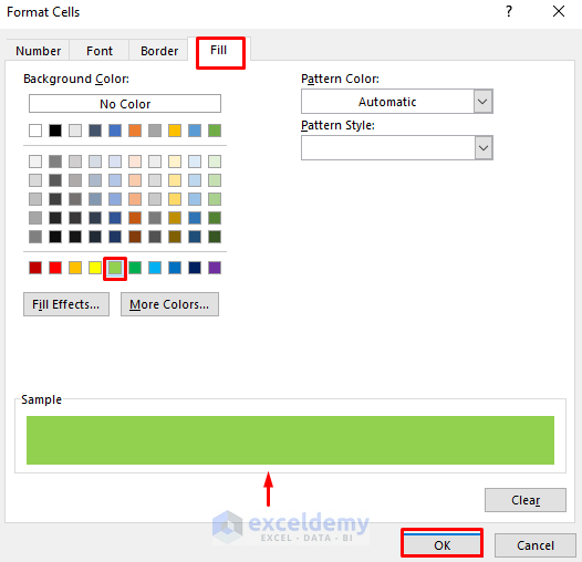
• The Format Cells dialog box will appear.
• Choose your desired color to fill the cells.
• Press OK.

• This will take you to the previous dialog box.
• Press OK.

• Go to Conditional Formatting and New Rule.
• Select between from the second drop-down.
• Type 5000 and 10000 in the third and fourth drop-downs, respectively.
• Choose the desired color from the Format Cells dialog box.
• Press OK.

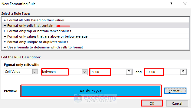
• We chose the blue color for the second condition.

• Repeat the above steps for the 3rd condition.
• Type 10000 and 15000 in the 3rd and 4th drop-downs.
• Select a different color.
• Press OK.

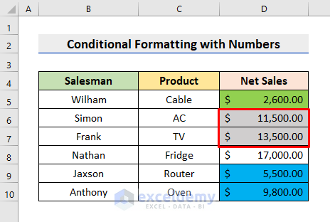
• We have added the third condition.

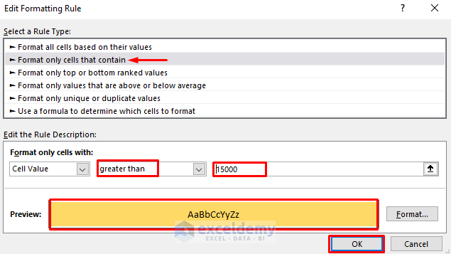
• Repeat the process for the last time.
• Select greater than from the second drop-down.
• Type 15000.
• Choose a color.
• Press OK.

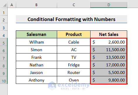
• You’ll see the Net Sales column in 4 different colors.

Read More: Excel Conditional Formatting Color Scale Based on Another Cell

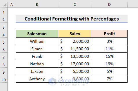
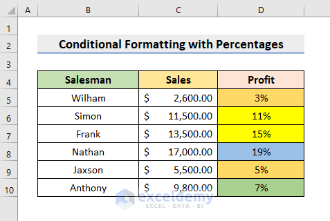
Method 2 – Apply a 4-Color Scale Conditional Formatting on Percentage Values

We’ll use the below dataset which has Profit percentages.

STEPS:

• Choose the range D5:D10.
• Select New Rule from the Conditional Formatting drop-down.

• If you want to apply the 3-Color Scale, select the Percent type as shown in the marked boxes.

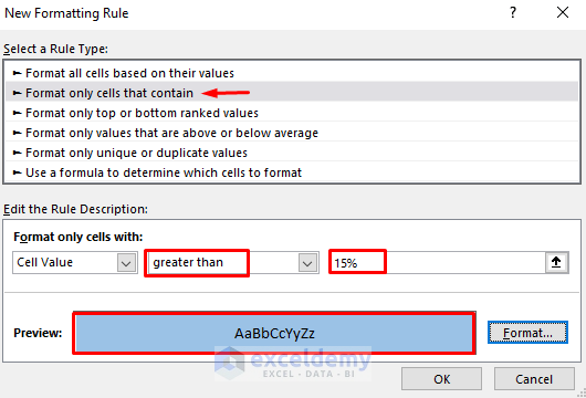
• To apply the 4-Color Scale, choose the 2nd Rule Type.
• Select less than or equal to from the 2nd drop-down.
• Type 5% in the 3rd box.
• Select the color from Format.
• Press OK.

• Repeat the above process.
• Use greater than.
• Type 15%.
• Select the color you wish.
• Press OK.

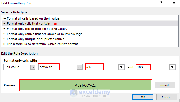
• Repeat the steps.
• Choose between.
• Type 6% and 10% in the boxes.
• Choose the color to fill the cells.
• Press OK.

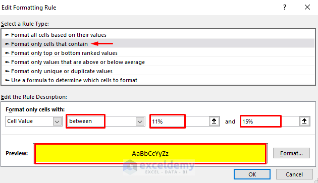
• Go through the process to apply the 4th color.
• Select between and type 11% and 15% in the boxes.
• After choosing a color, press OK.

• Each color denotes a specific criteria.

Read More: Conditional Formatting with 3 Color Scale in Excel Formula

Download the Practice Workbook

Related articles

• Color Scale Per Row with Conditional Formatting in Excel
• How to Use Conditional Formatting with 5 Color Scale in Excel
• How to Use Excel Color Scale Based on Text

<< Go Back to Conditional Formatting | Learn Excel