Assigning Weights to Variables in Excel (3 Useful Examples)

In many cases, the exams in a school, or products in a company carry equal weight or significance. In that case, the average is very easy to calculate. But, in some practical scenarios, the weights aren’t equivalent to each other. For that purpose, the weighted average is necessary to find out the average. But before that, we need to assign the weights to the variables. In this article, we’ll show you the practical examples of assigning weights to variables in Excel and thus calculate the weighted average.

3 Useful Examples of Assigning Weights to Variables in Excel

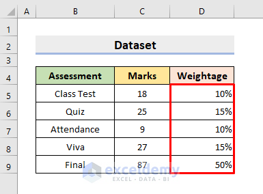
1. Assigning Weights to Variables in Excel When Total Weight Is 100%

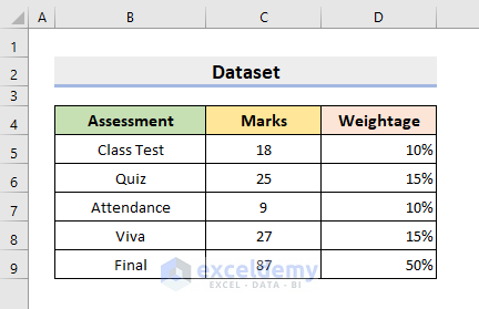
We know that various assessment systems prevail in educational institutions to evaluate the students’ performance. In our first example, we’ll assign the Weights to different types of exams present in a school. Here, in the following dataset, the Weightages add up to 100% in total. Therefore, follow the steps below to figure out the weighted average.

STEPS:

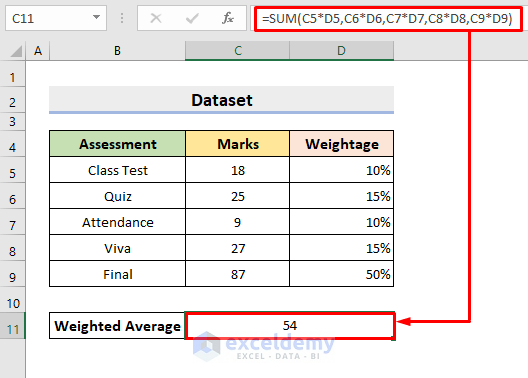
• First, select cell C11.
• Then, type the formula:

• After that, press Enter.
• Lastly, it’ll return the accurate value.

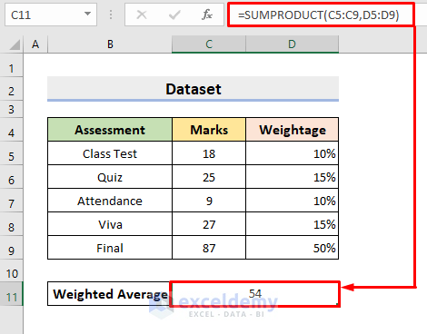
NOTE: The SUMPRODUCT function multiplies the C5:C9 array with the D5:D9 array at first. Next, it sums the product outputs.

Read More: How to Calculate Weighted Average with Percentages in Excel

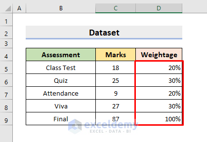
2. Allot Weights Whereas Total Weight Differs from 100%

However, there are some events where the Total Weight doesn’t add up to 100%. See the below dataset for Assigning Weights to variables in Excel and there, the total Weight is 200%. So, learn the following steps to compute the average.

STEPS:

• Firstly, select cell C11.
• Subsequently, type the formula:

• At last, press Enter and it’ll return the average.

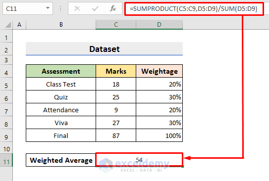
NOTE: At first, the SUMPRODUCT function multiplies the C5:C9 and D5:D9 array and then, sums the product outputs. After that, the result is divided by the output of the SUM function which finds the total of the D5:D9 array.

3. Use SUM Function to Assign Weights in Excel

In our last method, we’ll use the SUM function for Assigning Weights to variables in Excel and determine the weighted average. This process is a kind of a manual process. So, with a smaller dataset, we can apply this method without any difficulties. But, if we have to deal with a large number of data values, this process may not be a suitable option. Now, learn the steps given below to carry out the operation.

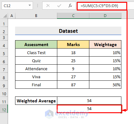
To illustrate, we’ll use the following dataset which is the same as the first 2 examples.

STEPS:

• Select cell C11 at first. Type the formula:

• Then, press Enter. It’ll return the precise result.

NOTE: The SUM function adds the products of the cells specified in the argument. Each cell is applied manually here.

Moreover, we can apply the function in another way to get the same output. For that, follow the below steps.

STEPS:

• Select cell C11 to type the formula:

• Eventually, press Enter.

Here, inside the SUM function argument, we are multiplying the arrays C5:C9 and D5:D9 at first.

Download Practice Workbook

Download the following workbook to practice by yourself.

Conclusion

Henceforth, you will be able to carry out the operation for assigning weights to variables in Excel following the above-described examples. Keep using them and let us know if you have any more ways to do the task.

Related Articles

• Calculate Weighted Average Price in Excel
• How to Calculate Weighted Moving Average in Excel
• Calculate Conditional Weighted Average with Multiple Conditions in Excel

<< Go Back to Weighted Average Excel | How to Calculate Average in Excel | How to Calculate in Excel | Learn Excel