Calculate Conditional Weighted Average with Multiple Conditions in Excel

This tutorial will demonstrate the methods to calculate conditional weighted average with multiple conditions in Excel. While calculating the weighted average we might need to calculate only for specific instances of our dataset. So, we have to apply conditions to get our desired result. We can use the generic method to apply conditions manually. But this method is not feasible while we will be working with a large dataset. To overcome this situation we will use different Excel functions to apply multiple conditions to calculate the weighted average.


What Is Weighted Average in Excel?

Weighted average in Excel refers to the arithmetic mean. Here, certain data elements are always more important than others. If we say it in another way, every value that we will average has a specific weight.


Calculate Conditional Weighted Average with Multiple Conditions in Excel: 5 Easy Methods

Throughout this article, we will discuss 5 easy methods to calculate conditional weighted average in Excel. All methods will with multiple conditions. To illustrate the methods we will use the following dataset. The dataset contains two types of food fruit and vegetable with their Quantity and Average Price. Suppose, we want to calculate the weighted average only for the food type Fruit. To do this, we need to apply conditions that will return only the weighted average for Fruit.

5 Easy Methods to Calculate Conditional Weighted Average with Multiple Conditions in Excel


1. Use Generic Formula Calculate Conditional Weighted Average with Multiple Conditions in Excel

In the first method, we will use the generic formula to calculate the conditional average with multiple conditions. We may call it a manual way.

GENERIC FORMULA:

Weighted Average = (Sum of Weighted Terms)/(Total Number of Terms)

Let’s see the steps to perform this method.

STEPS:

  • To begin with, select cell F13.
  • In addition, type the following formula in that cell:
=(F5+F6+F9)/(D5+D6+D9)
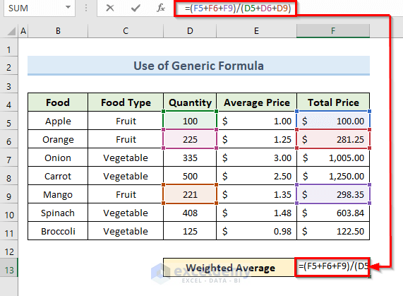
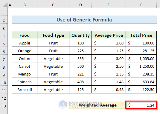
Use Generic Formula Calculate Conditional Weighted Average with Multiple Conditions in Excel

  • Then, press Enter.
  • Finally, we get a result like the following image. The value of $1.24 in cell F13 indicates the weighted average only for the food type Fruit.

Read More: How to Calculate Weighted Average Price in Excel


2. Utilize Only SUMIFS Function to Enumerate Conditional Weighted Average with Various Conditions.

In the second method, we will use the SUMIFS function to calculate the conditional weighted average with various conditions. The SUMIFS function in Excel calculates the total of cells that satisfy multiple conditions. To apply conditions using the SUMIFS function follow the below steps.

STEPS:

  • First, select cell F13.
  • Next, insert the following formula in that cell:
=SUMIFS(F5:F11,C5:C11,"*Fruit*")/SUMIFS(D5:D11,C5:C11,"*Fruit*")
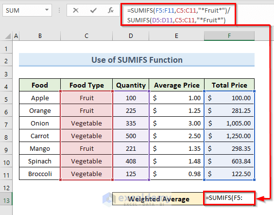
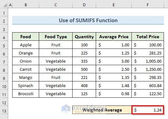
Utilize Only SUMIFS Function to Enumerate Conditional Weighted Average with Various Conditions.

  • Then, hit Enter.
  • As a result, we get the value of the weighted average for food type Fruit in cell F13.


3. Calculate Conditional Weighted Average with Multiple Conditions Using Table Format

In this method, we will use the table format of our dataset to calculate the conditional weighted average. Also, we will use multiple conditions to do this. We will use the combination of the SUMIF function and Table Reference formula for this method too. In the table format of our previously mentioned dataset follow the below steps.

STEPS:

  • Firstly, select cell F13.
  • Secondly, input the following formula in that cell:
=SUMIF(Table2[Food Type],B14,Table2[Total Price])/SUMIF(Table2[Food Type],B14,Table2[Quantity])
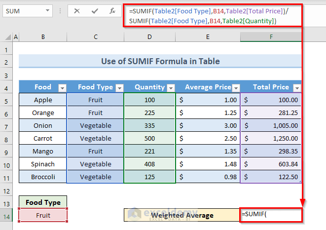
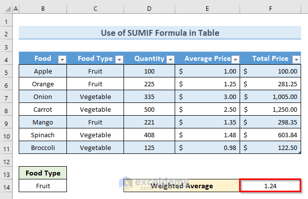
Calculate Conditional Weighted Average with Multiple Conditions Using Table Format

  • Press Enter.
  • Lastly, we can see the value of the weighted average in cell F13.


4. Combine SUMPRODUCT and SUMIF Functions to Calculate Conditional Weighted Average

Another way to calculate the conditional weighted average is to use a combination of the SUMPRODUCT and SUMIF functions. The SUMPRODUCT function in Excel calculates the sum of the products of two or more ranges or arrays. By default this function does multiplication. But we can also do addition, subtraction, and division. To use these functions to calculate the conditional weighted average we will follow the below simple steps.

STEPS:

  • In the beginning, select cell E13.
  • Next, type the following formula in that cell:
=SUMPRODUCT((C5:C11="Fruit")*D5:D11*E5:E11)/SUMIF(C5:C11,"Fruit",D5:D11)
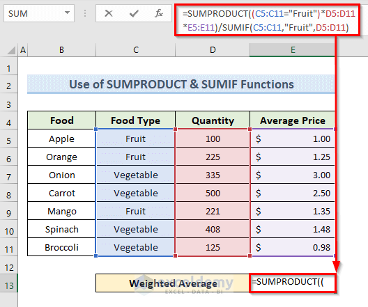
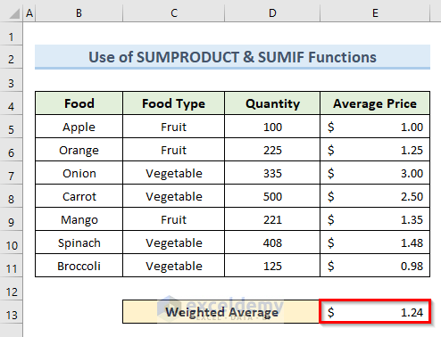
Combine SUMPRODUCT and SUMIF Functions to Calculate Conditional Weighted Average

  • Press Enter.
  • In the end, we get the value of the weighted average for fruits in cell E13.

Here, the SUMPRODUCT function returns the product of quantity and average price for the food type Fruit only. The SUMIF function returns the sum of the quantity of food type Fruit.


5. Estimate Weighted Average with Multiple Conditions with SUMPRODUCT, ISNUMBER & SEARCH Functions

We can also calculate conditional averages with multiple conditions using the SUMPRODUCT, ISNUMBER, and SEARCH functions.

The ISNUMBER function determines whether a cell in Excel has a number or not. If the value is a number, it will return TRUE. Otherwise, it will return FALSE.

The SEARCH function in Excel returns the location of one text string within another one. If the search string appears more than once, the SEARCH function returns the position of the first encounter.

So, let’s see the steps to perform this method.

STEPS:

  • To begin with, select cell E13.
  • In addition, enter the following formula in that cell:
=SUMPRODUCT((ISNUMBER(SEARCH("Fruit",C5:C11))*(D5:D11)*(E5:E11)))/SUMPRODUCT((ISNUMBER(SEARCH("Fruit",C5:C11))*(D5:D11)))
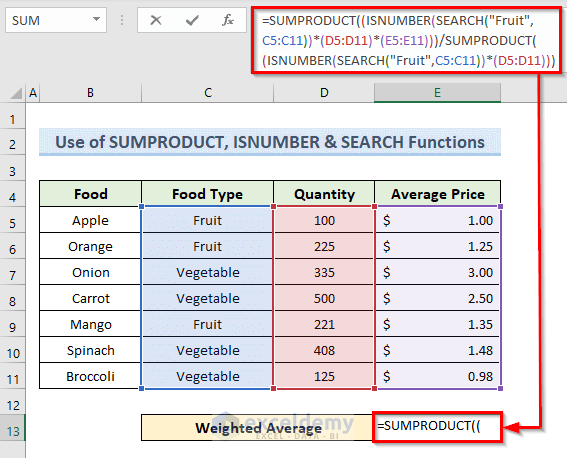
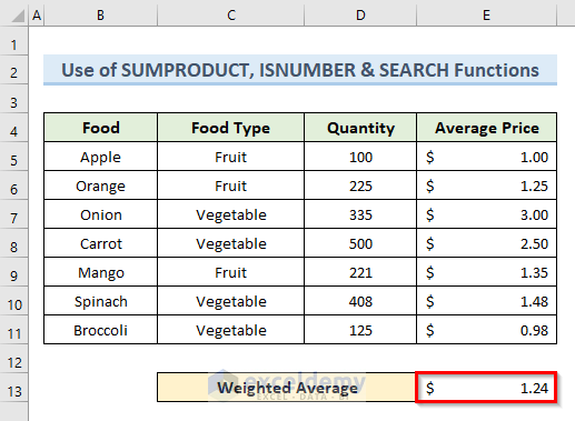
Estimate Weighted Average with Multiple Conditions with SUMPRODUCT, ISNUMBER & SEARCH Functions

  • Hit, Enter.
  • Lastly, we can see the result in the following image. The above formula returns the value of the weighted average for food type Fruit in cell E13.

🔎 How Does the Formula Work?

  • SEARCH(“Fruit”,C5:C11): In this part, the SEARCH function searches for the string Fruit within cell range C5 to C11.
  • ISNUMBER(SEARCH(“Fruit”,C5:C11)): Here, the ISNUMBER function checks whether the value we are searching for is a number or not.
  • SUMPRODUCT((ISNUMBER(SEARCH(“Fruit”,C5:C11))*(D5:D11)*(E5:E11))): This part returns the product of the specified ranges for the food type Fruit.
  • SUMPRODUCT((ISNUMBER(SEARCH(“Fruit”,C5:C11))*(D5:D11))): Here the SUMPRODUCT function returns the sum of quantity for the food type Fruit.
  • SUMPRODUCT((ISNUMBER(SEARCH(“Fruit”,C5:C11))*(D5:D11)*(E5:E11)))/SUMPRODUCT((ISNUMBER(SEARCH(“Fruit”,C5:C11))*(D5:D11))): This part calculates the weighted average for the food type Fruit.

Download Practice Workbook

You can download the practice workbook from here.


Conclusion

In conclusion, this tutorial shows five effective methods to calculate conditional weighted average. In addition, we have used use multiple conditions to do that. So, put your skills to the test with the practice worksheet included in this article. Please leave a comment in the box below if you have any questions. We’ll do everything we can to react as quickly as possible.


Related Articles


<< Go Back to Weighted Average Excel | How to Calculate Average in Excel | How to Calculate in Excel | Learn Excel

Get FREE Advanced Excel Exercises with Solutions!
Mukesh Dipto
Mukesh Dipto

Mukesh Dipto is an excellent marine engineer who loves working with Excel and diving into VBA programming. For him, programming is like a superhero tool that saves time when dealing with data, files, and the internet. His skills go beyond the basics, including Rhino3D, Maxsurf C++, AutoCAD, HTML, CSS, JavaScript, and WordPress. He got his B.Sc in Naval Architecture & Marine Engineering from BUET, and now he's switched gears, working as a content developer. In this role, he... Read Full Bio

We will be happy to hear your thoughts

Leave a reply

Advanced Excel Exercises with Solutions PDF


ExcelDemy
Logo