How to Calculate Weighted Average with Percentages in Excel

While calculating a weighted average, the weights of each data point are often expressed in percentages. In the following image, we have varying weights for each data point and these weights are expressed in percentages. We will calculate the weighted average here.

Note: We used Excel for Microsoft 365 to prepare this article. However, you can find the functions used in this tutorial in Excel 2021, Excel 2019, Excel 2016, Excel 2013, Excel 2010, and Excel 2007 versions as well.

What Is the Weighted Average?

You can use the following formula to calculate a weighted average.

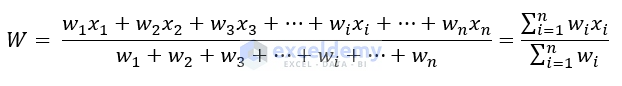
W = weighted average

n = number of terms to be averaged

x_i = data points to be averaged

w_i = weights applied to corresponding x_i values

How to Calculate the Weighted Average in Excel

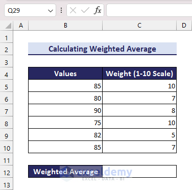
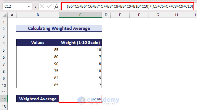
Consider the following dataset. We have a few values and their weights. We have taken weights from 1 to 10 scale, but they can be any.

• In cell C12, insert the following formula.

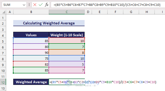
We have multiplied each value with the corresponding weight, summed the products, and divided the result with the sum of the weights.

• Press the Enter key.

Method 1 – Calculating the Weighted Average with Percentages Using an Arithmetic Formula in Excel

Consider the following dataset where we have a student score out of 100 in Quiz, Assignment, Project, Mid Term Exam, and Term Final Exam. All these items carry different weights (expressed in percentages). We will use the arithmetic formula to calculate the weighted average score of this student here.

Steps:

• Insert the following formula in cell C12.

• Press the Enter key.

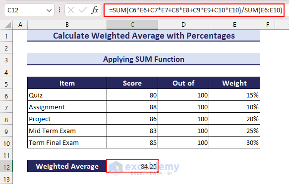
Method 2 – Applying the SUM Function to Calculate the Weighted Average with Percentages in Excel

Steps:

• Apply the following formula in cell C12.

• Press the Enter key.

Note: If the weights add up to 100% i.e. 1, you can skip dividing with the sum of weights. In our dataset, the weight adds up to 100% (15% + 10% + 20% + 25% + 30% = 100%). So the following formula will return the same result as the previous two methods.

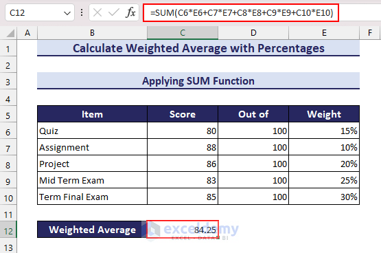
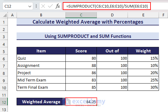
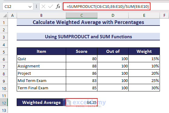
Method 3 – Using SUMPRODUCT and SUM Functions to Calculate the Weighted Average with Percentages in Excel

Steps:

• Insert the following formula in cell C12.

• Press the Enter key.

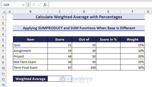
Method 4 – Applying SUMPRODUCT and SUM Functions to Calculate the Weighted Average with Percentages (When the Base Is Different)

In previous methods, we measured the scores of each item out of 100. But the base can be different as well.

Consider the following dataset. The scores of each item are measured out of different values. To calculate the weighted average in this case, we require an additional column to calculate the percentage of score for each score. This will make the base of each score equal.

Steps:

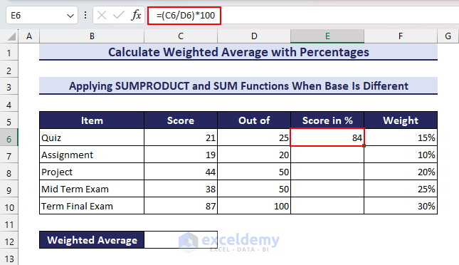
• Insert the following formula in cell E6.

• Press the Enter key.

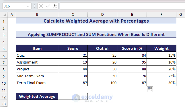
• Hover your mouse pointer over the bottom-right corner of cell E6. You will find the Fill Handle icon.

• Double-click on the Fill Handle icon to obtain the percentage score for all items.

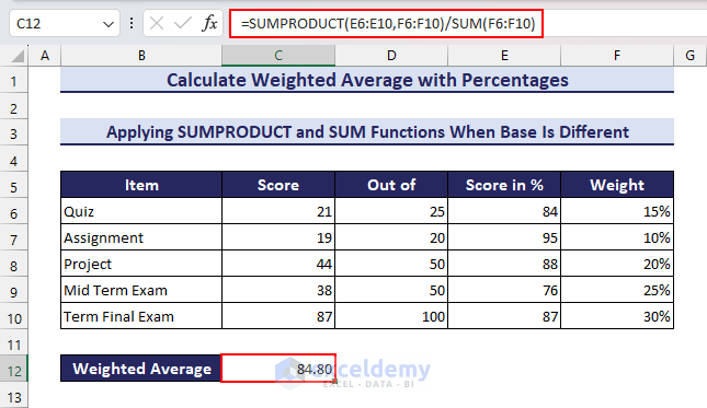
• Apply the following formula in cell C12.

• Press the Enter key and you will get the required weighted average score.

Read More: Assigning Weights to Variables in Excel

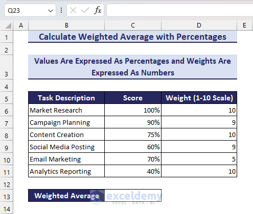
Method 5 – Calculate the Weighted Average When Values Are Expressed as Percentages and Weights Are Expressed as Numbers in Excel

The scores are in percentages and the weights are in numbers here.

Steps:

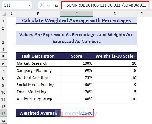
• Insert the following formula in cell C13.

• Press the Enter key.

Calculate the Weighted Average with Percentages in Excel for Real World Scenarios

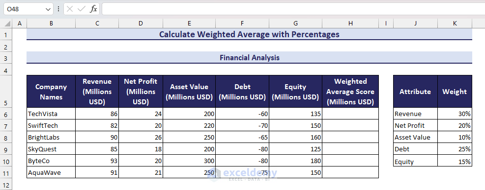
Example 1 – Financial Analysis

Consider the following dataset. We have Revenue, Net Profit, Asset Value, Debt, and Equity values of a few companies. We also have the weight percentages (i.e. significance) of each attribute.

Steps:

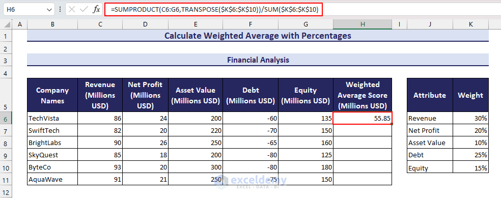
• In cell H6, apply the following formula.

Since the attribute values are in a row and weights are in a column, we have used the TRANSPOSE function here to take the weights in a row as well.

• Press the Enter key.

• Use the Fill Handle feature.

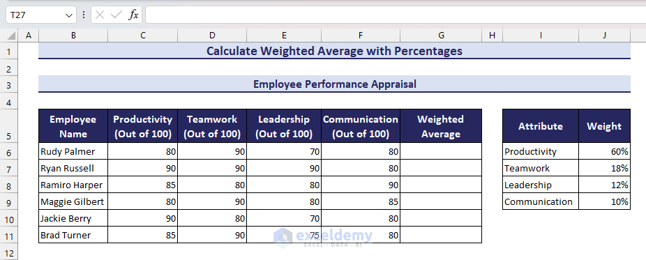
Example 2 – Employee Performance Appraisal

Consider the following dataset. We have listed the Productivity, Teamwork, Leadership, and communication scores (out of 100) of a few employees. We also have the weight percentages (i.e. importance) of these attributes.

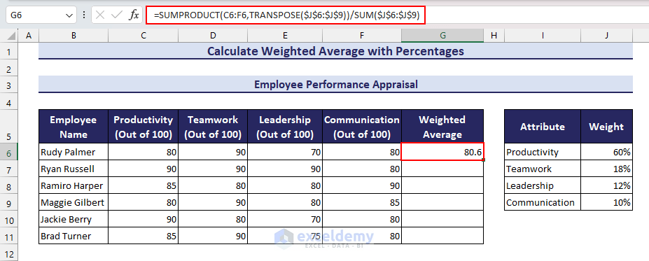
Steps:

• Insert the following formula in cell G6.

• Press the Enter key.

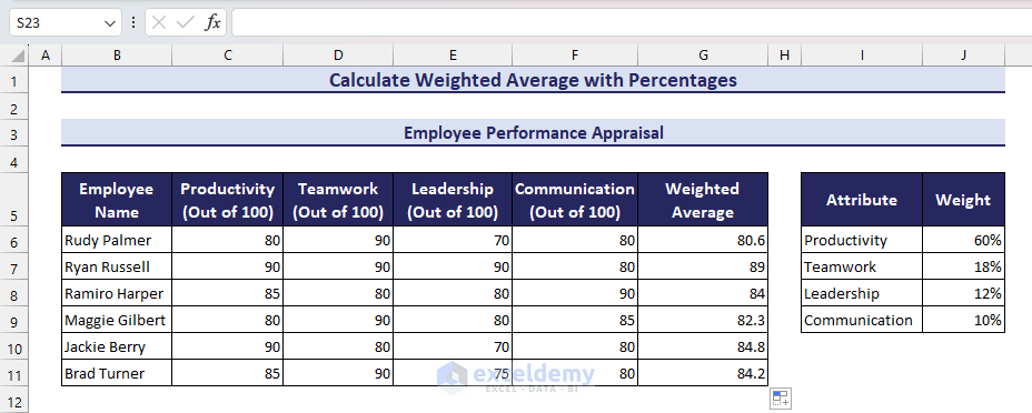
• Drag down the Fill Handle tool to obtain the weighted average score for all employees.

Download the Practice Workbook

Related Article

• Calculate Conditional Weighted Average with Multiple Conditions in Excel

<< Go Back to Weighted Average Excel | How to Calculate Average in Excel | How to Calculate in Excel | Learn Excel