Excel Formula to Compare Two Columns and Return a Value (5 examples)

Method 1 Compare Two Columns and Return a Value from the Second Column with the VLOOKUP Formula

In the following spreadsheet, we have a list of Projects and their Managers. In cell D2, the Project coordinator might input a Project name and want to see who the Manager of the Project is.

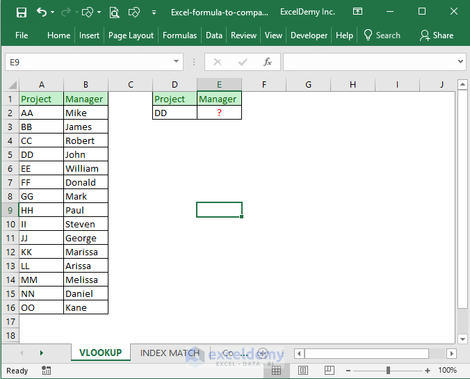
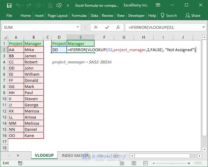
• Use this formula in cell E2: =IFERROR(VLOOKUP(D2,project_manager,2,FALSE), “Not Assigned”)

How does this formula work?

To understand this formula, you have to know the syntax of IFERROR and VLOOKUP Excel functions.

Here’s how the formulas join together to get a result.

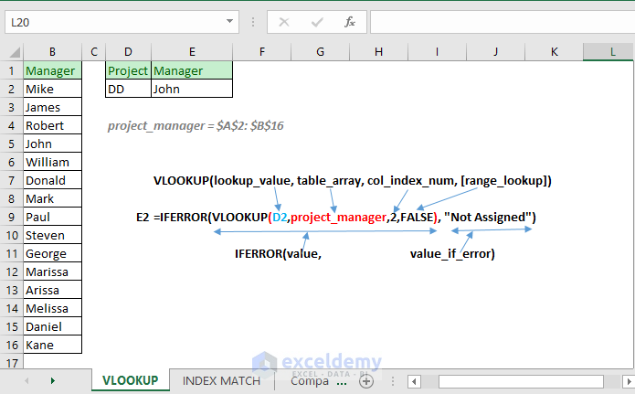
Here’s a full review of what each part does.

Read More: How to Match Two Columns and Return a Third in Excel

Method 2 – Compare Two Columns and Return a Value (using INDEX and MATCH functions)

• Use the following formula for cell E2: =IFERROR(INDEX(B2:B16, MATCH(D2,A2:A16,0)), “”)

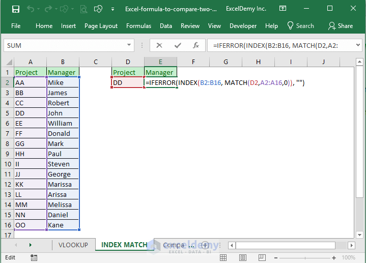
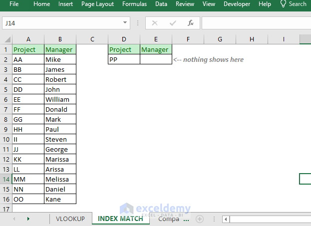
If the formula doesn’t find a match, it won’t return a value since the IFERROR function’s value_if_error argument is blank.

How does the formula work?

Check out the following image.

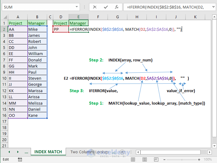
Here’s how the formula works in steps:

• The MATCH function returns the relative position of lookup_value D2. Say, the value is DD. It will return 4 as DD is in 4^th position in the lookup_array $A$2:$A$16. If no matching was found, the MATCH function would return an error value.
• The INDEX function searches for the 4^th value in the array $B$2:$B$16. And it finds value, John. So, for this example, the INDEX function will return the value, John.
• The IFERROR function finds a valid value for its value So, it will return the value. If it would find an error value, then it would return a blank.

Read More: How to Count Matches in Two Columns in Excel (5 Easy Ways)

Method 3 – Two Columns Lookup

Here’s a dataset of employees and their salaries. We’ll find a salary for an employee with a given first and last name.

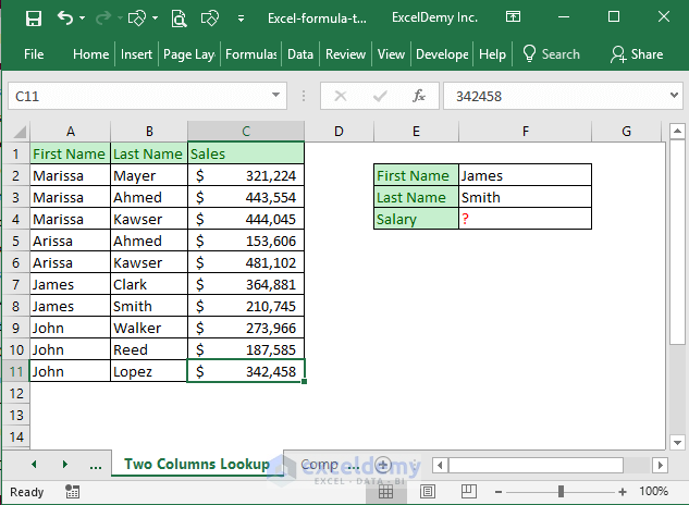
You cannot perform two columns lookup with regular Excel formulas. You have to use an Array formula.

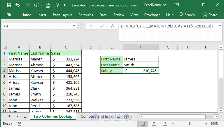
• Input this formula in cell F4: {=INDEX(C2:C11,MATCH(F2&F3, A2:A11&B2:B11,0))}

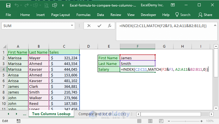
• Press Ctrl + Shift + Enter on your keyboard. You will get the formula as an array formula.

How does this array formula work?

At first, let’s understand the Match function part.

You can imagine this array formula as a series of the following formulas:

• MATCH(F2&F3, A2&B2,0)
• MATCH(F2&F3, A3&B3,0)
• MATCH(F2&F3, A4&B4,0)
• … … …
• … … …
• MATCH(F2&F3, A11&B11,0)

This series will be stored in Excel memory as <code>MATCH (JamesSmith, {“MarissaMayer”; “MarissaAhmed”; “MarissaKawser”; “ArissaAhmed”; “ArissaKawser”; “JamesClark”; “JamesSmith”; “JohnWalker”; “JohnReed”; “JohnLopez”}, 0)

From the above MATCH function, what will be returned? MATCH function will return 7 as JamesSmith is found at position 7 of the array.

The rest is simple. In the array of C2:C11, the 7^th position is value 210745. So, the overall function returns 210745 in cell F4.

Read More: How to Compare Text Between Two Cells in Excel (10 Methods)

Similar Readings

• How to Compare Two Columns in Excel for Missing Values (4 ways)
• Match Two Columns and Output a Third in Excel (3 Quick Methods)
• Excel Formula to Compare and Return Value from Two Columns
• Excel Macro to Compare Two Columns (4 Easy Ways)
• How to Match Multiple Columns in Excel (Easiest 5 ways)

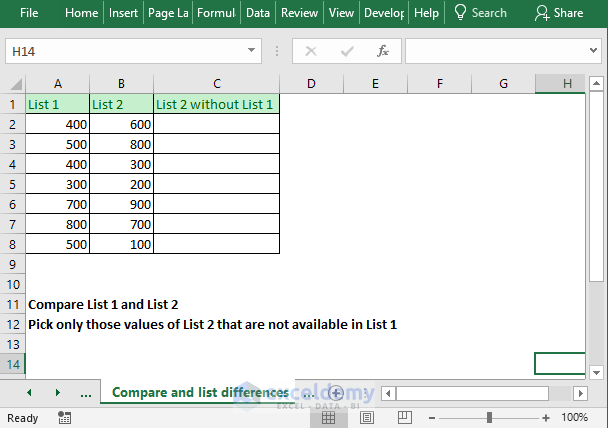
Method 4 – Compare Two columns and List Differences in the Third Column

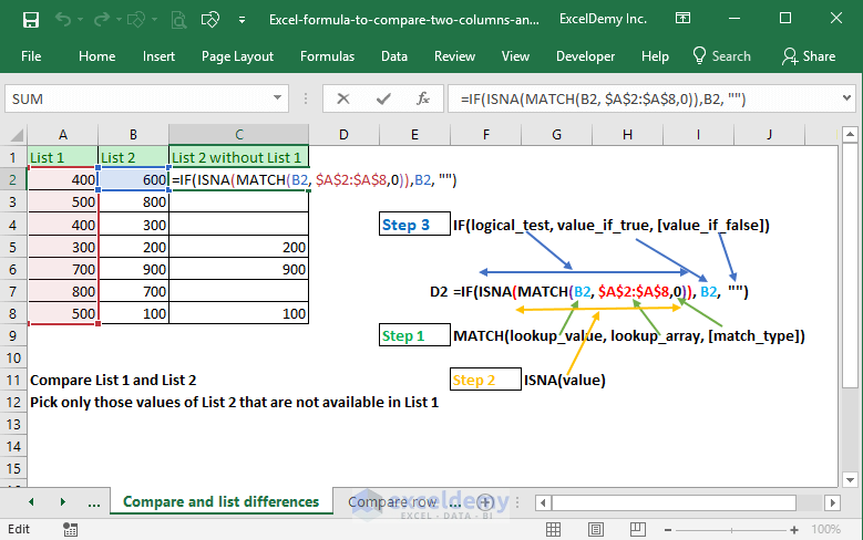
Here are two lists that we need to compare and show the values of List 2 under a new column but without the values that are also in List 1.

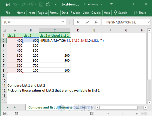
• Use this formula in cell C2: =IF(ISNA(MATCH(B2, $A$2:$A$8,0)),B2, “”)
• Drag the formula down to copy it for the other cells.
• We get the following results for the sample.

How does this formula work?

Let’s break down the formula into pieces:

• The Match function will search for cell value B2 in the range $A$2:$A$8. If it finds a match, it will return the position of the value, otherwise, it will return the #N/A. Value 600 of cell B2 is not found anywhere on the list. So, the Match function will return the #N/A error.
• The ISNA function returns TRUE if it finds the #N/A error, otherwise, it will return a FALSE In this case, ISNA will return TRUE value as Match function returns #N/A error.
• When the ISNA function returns a TRUE value, IF function’s value_if_true argument will be returned and it is B2, the value of B2 is 600. So, this formula will return 600 as a value.

Read More: How to Compare Two Lists and Return Differences in Excel

Method 5 – Compare Two Columns Row by Row

You might also want to compare two columns row by row like the following image.

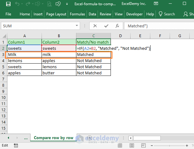
• Use the following formula in cell C2: =IF(A2=B2, “Matched”, “Not Matched”)
• AutoFill to the other cells in the result column.

This is a straightforward Excel IF function. If the cells A2 and B2 are the same, “Matched” value will show in cell C2 and if the cells A2 and B2 are not the same, then the “Not Matched” value will show as the output.

This comparison is case-insensitive. “Milk” and “milk” are treated as the same in this comparison.

• We can also use the EXACT function to find the exactly matched values. Change the formula to the following: =IF(EXACT(A2,B2), "Matched", "Not Matched")

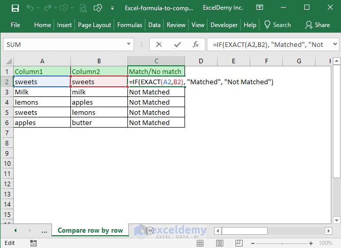
You see now “Milk” and “milk” are treated differently. They are not the same.

Read More: How to Compare Text in Two Columns in Excel

Download the Working File

Further Readings

• How to Compare Two Columns or Lists in Excel (4 Suitable Ways)
• VLOOKUP Formula to Compare Two Columns in Different Excel Sheets
• How to Compare Two Columns for Finding Differences in Excel
• Compare Two Columns in Excel and Highlight the Greater Value (4 Ways)
• How to Compare Multiple Columns Using VLOOKUP in Excel (5 Methods)