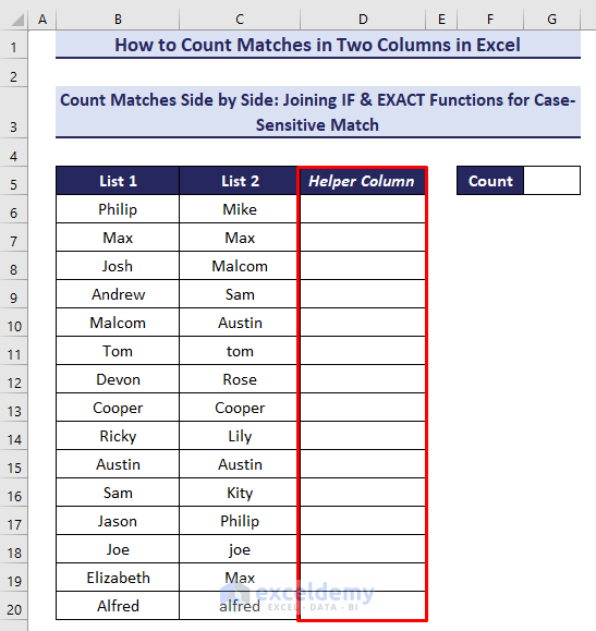
Suppose you have the following dataset.
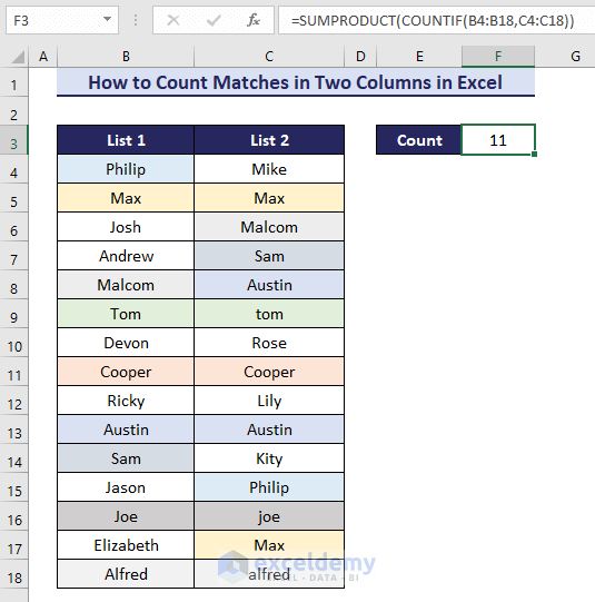
Watch Video – Count Matches in Two Columns in Excel
Method 1 – Count Matches in Two Columns (Match Side-by-Side)
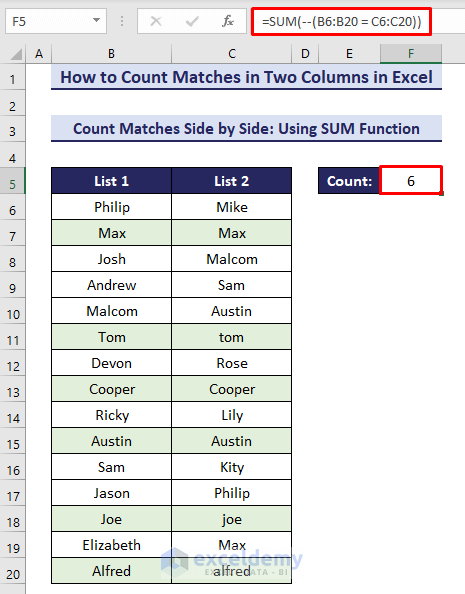
Using the SUM Function
Steps:
- Insert the following formula in the relevant cell (F5 in this example).
=SUM(--(B6:B20 = C6:C20))- Hit Enter.
- Use the following formula to apply conditional formatting to the chosen cells.
=$B6=$C6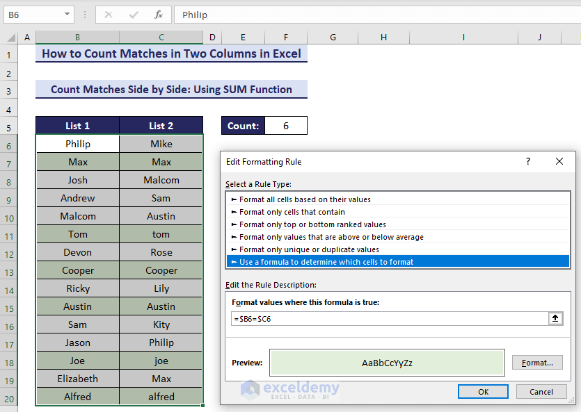
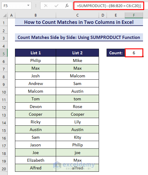
Using the SUMPRODUCT Function
Steps:
- Insert the following formula in the relevant cell (F6 in this example).
=SUMPRODUCT(--(B6:B20 = C6:C20))- Hit Enter.
Combining Excel EXACT and IF Functions for Case-Sensitive Match
Steps:
- Add a helper column to use these functions.
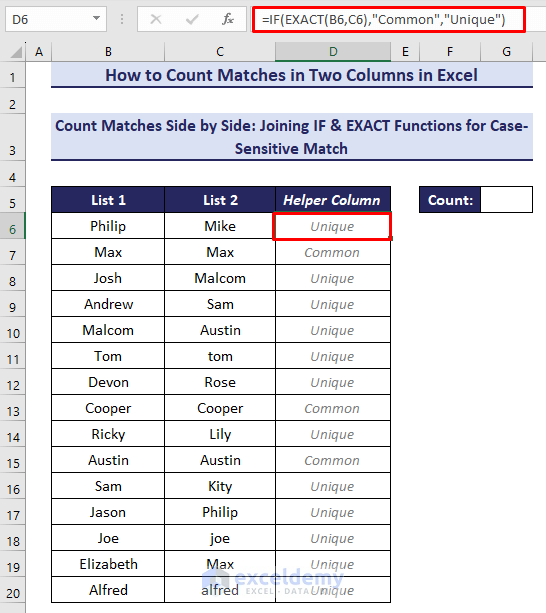
- Use the following formula in the relevant cell (D6 in this example).
=IF(EXACT(B6,C6),"Common","Unique")- Use the Auto Fill tool to copy the formula to the other cells of the column.
This formula will return ‘Unique’ if it doesn’t get exact values with the same case, and return ‘Common’ if it gets exact values with the same case.
- Use the following formula to count the matching values.
=COUNTIF(D6:D20,"Common")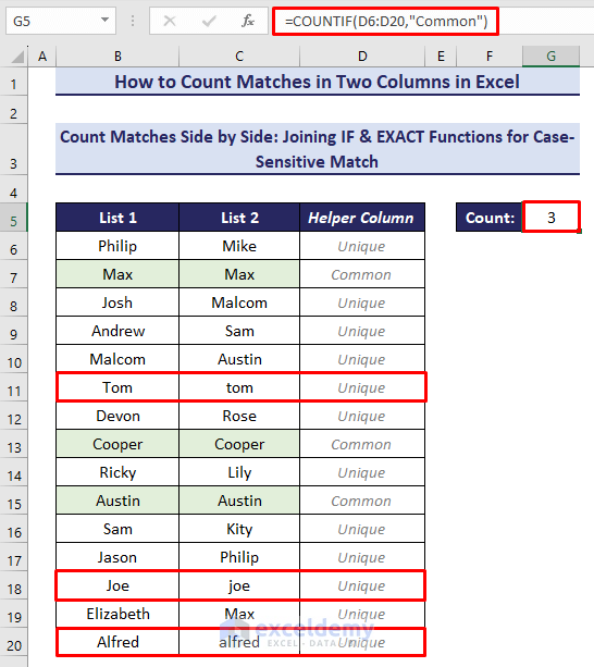
Method 2 – Count Matches in Two Columns (Not Side by Side)
Combining Excel SUMPRODUCT & COUNTIF Functions
Steps:
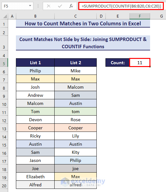
- Insert the following formula in the relevant cell (F6).
=SUMPRODUCT(COUNTIF(B6:B20,C6:C20))- Press Enter.
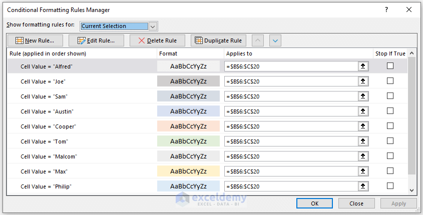
- Use individual conditional formatting to highlight duplicates of each item with different colors.
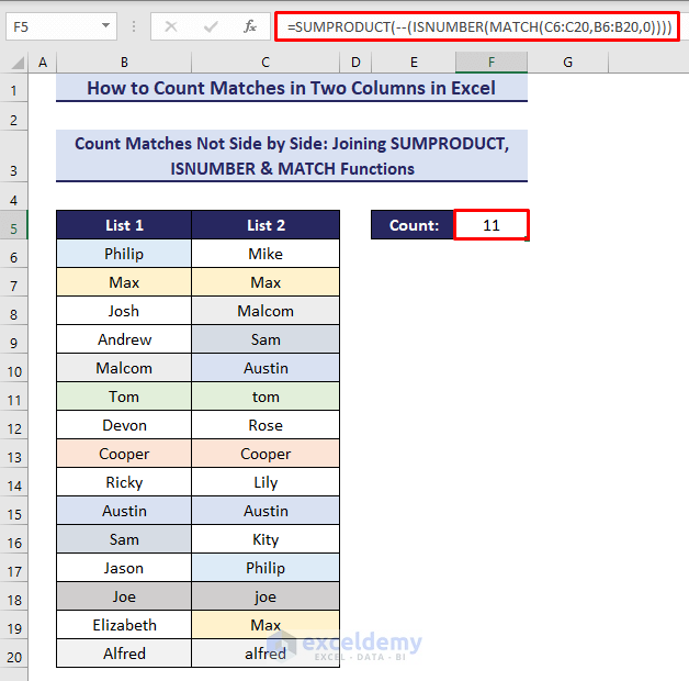
Merging Excel SUMPRODUCT, ISNUMBER & MATCH Functions
Steps:
- Insert the following formula in the relevant cell (F6).
=SUMPRODUCT(--(ISNUMBER(MATCH(C6:C20,B6:B20,0))))- Press Enter.
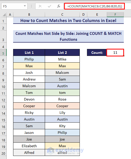
Joining the COUNT & MATCH Functions
Steps:
- Insert the following formula in the relevant cell (F6).
=COUNT(MATCH(C6:C20,B6:B20,0))- Press Enter.
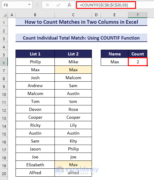
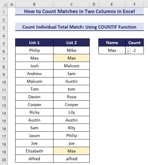
Method 3 – Count Individual Total Match
Steps:
- Insert the following formula in the relevant cell (F6).
=COUNTIF($C$6:$C$20,E6)- Press Enter.
- Use conditional formatting to highlight the matches.
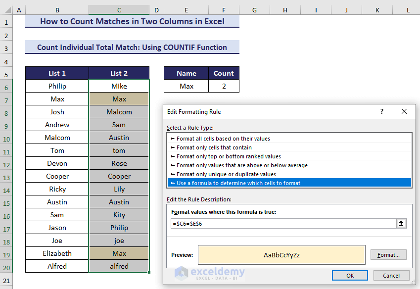
- Create a drop-down list for a more dynamic selection of the results.
Download Practice Workbook
You can download our free practice workbook to practice the methods.
<< Go Back to Columns | Compare | Learn Excel
Get FREE Advanced Excel Exercises with Solutions!
