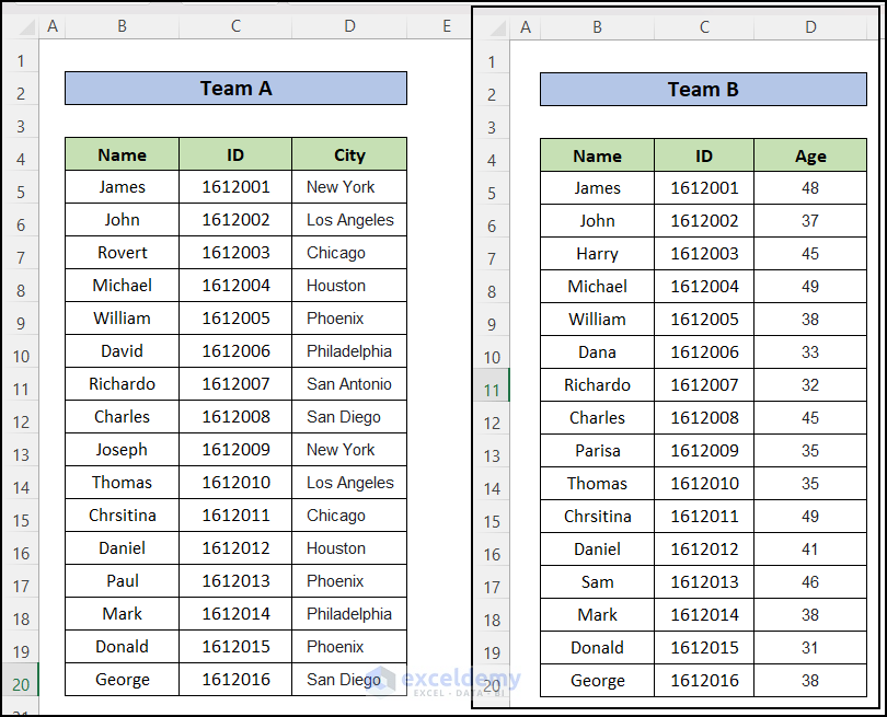
We have data from two teams that have some common members in two different worksheets named TeamA and TeamB. We’ll find the common names and the different names of the two teams.
Method 1 – Compare Two Columns in Different Excel Sheets and Return Common or Matched Values
- We have created a new worksheet with data of Team B.
- Create a new column E to find the common names.
- Insert the following formula into cell E5:
=VLOOKUP(B5,TeamA!B5:B20,1,FALSE)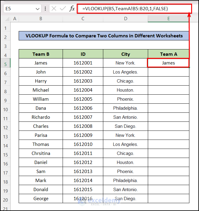
- Drag the Fill Handle icon down.
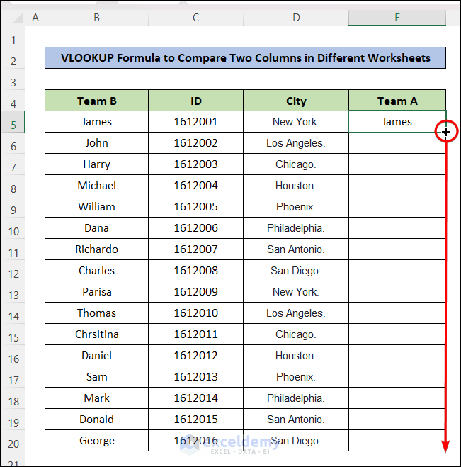
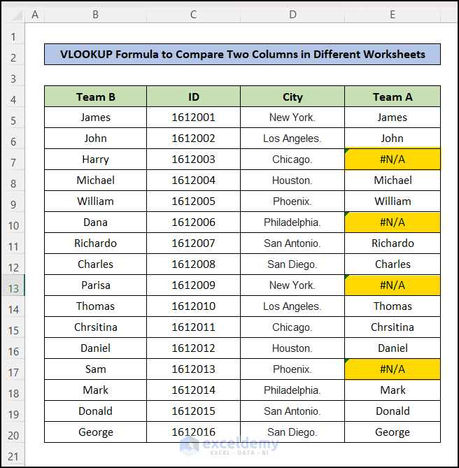
- You will get the common names inserted in the column Team A. For the mismatched rows, you’ll get an #N/A Error.
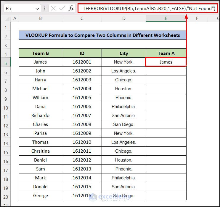
Using IFERROR with VLOOKUP Function to Treat the #N/A Error
To avoid the showing of ‘#N/A Error” in the column, use the following formula instead:
=IFERROR(VLOOKUP(B5,TeamA!B5:B20,1,FALSE),"Not Found")Formula Breakdown:
The syntax of IFERROR function: =IFERROR(value, value_if_error)
- As the value of IFERROR function, we have input our VLOOKUP. So, if there is no error, the output of the VLOOKUP formula will be the output of the IFERROR function.
- As the value_if_error argument, we have passed this value, “Not Found”. If the IFERROR function finds an error in the cell, it will output this text, “Not Found”.
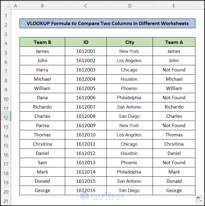
- Here’s the updated result.
Using IF and ISNA with VLOOKUP Function to Handle the #N/A Error:
=IF(ISNA(VLOOKUP(B5,TeamA!B5:D20,1,FALSE)),"Not Matched", "Matched")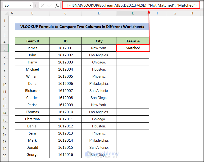
Formula Breakdown:
- ISNA returns a TRUE value if its argument is a N/A error, which is then used for the IF function.
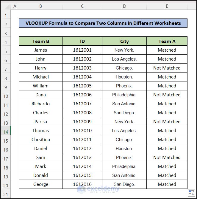
- Here’s the result of the new formula.
- Go back to the formula that outputs the names as results.
- Click on any cell of the dataset.
- Go to the Home tab on the top ribbon.
- Click on the Sort & Filter option and select Filter.
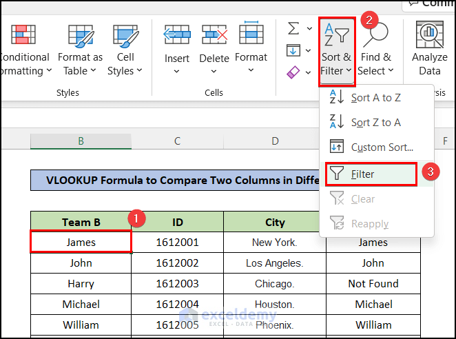
- You will filter drop-down arrows in each header of the dataset.
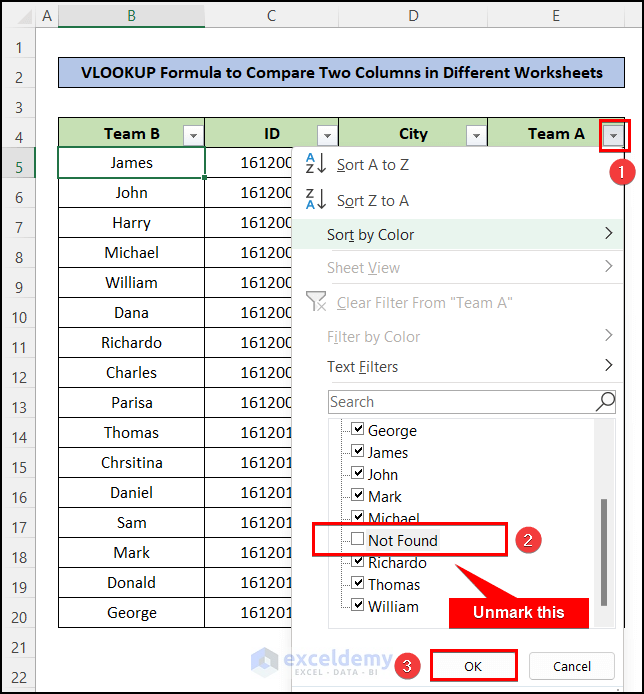
- Click on the Filter arrow in the Column Team A.
- Unmark the checkbox “Not Found” and press OK.
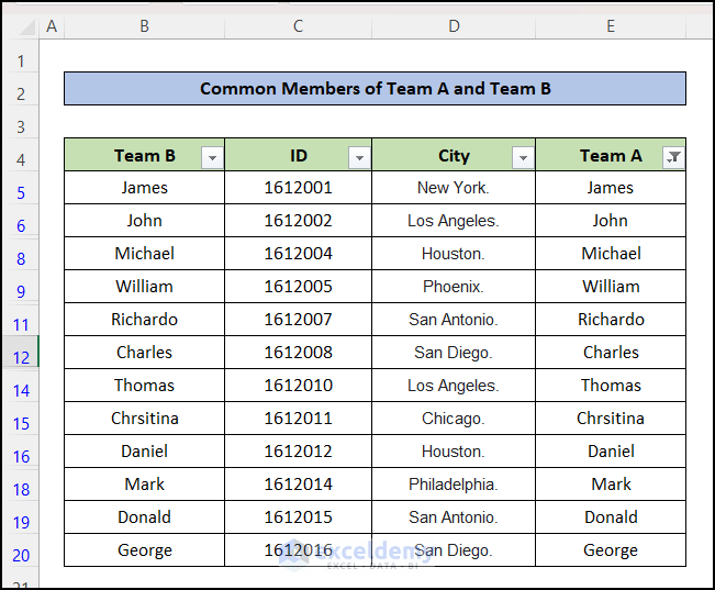
- You will see only the common or matched names of the two teams. Mismatched names are hidden by the Filter Feature.
Method 2 – Compare Two Columns in Different Worksheets and Find Missing Values
Case 2.1 – Using the Filter Feature
- Use the VLOOKUP formula with the IFERROR function from Method 1.
- Go to the Filter option by clicking the Filter arrow in the column header of Team A.
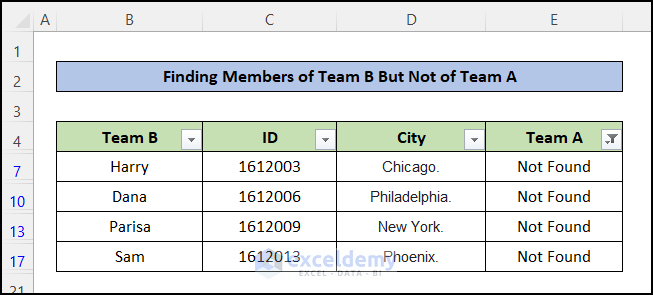
- Unmark all the checkboxes except that saying “Not Found”.
- Press OK.
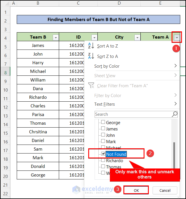
- You will see that only the mismatched names of Team B compared to Team A are shown in the dataset.
Case 2.2 – Using FILTER with VLOOKUP Function
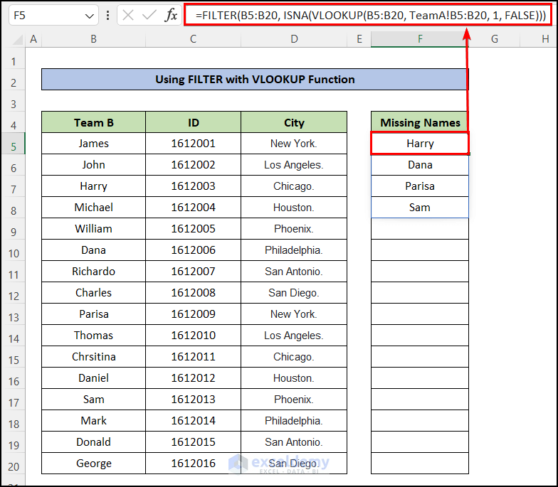
- Insert the following formula into cell F5.
=FILTER(B5:B20, ISNA(VLOOKUP(B5:B20, TeamA!B5:B20, 1, FALSE)))Formula Breakdown:
- The VLOOKUP function will find the common names between the range B5:B20 of the active worksheet and range B5:B20 of the worksheet TeamA and assign #N/A for the mismatched.
- The ISNA function will take only the cells that are assigned #N/A by VLOOKUP functions which means they are mismatched.
- The Filter function will insert only the cells from range B5:B20 which are mismatched and assigned #N/A.
Method 3 – Compare Two Lists in Different Worksheets and Return a Value from a Third Column+
- Change the column index number in the VLOOKUP. We want to get the age of the name “James” and the age values are contained in the 4th column of the selected VLOOKUP range in the TeamB worksheet.
- Insert the following formula into the cell E5:
=FILTER(B5:B20, ISNA(VLOOKUP(B5:B20, TeamA!B5:B20, 1, FALSE)))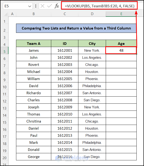
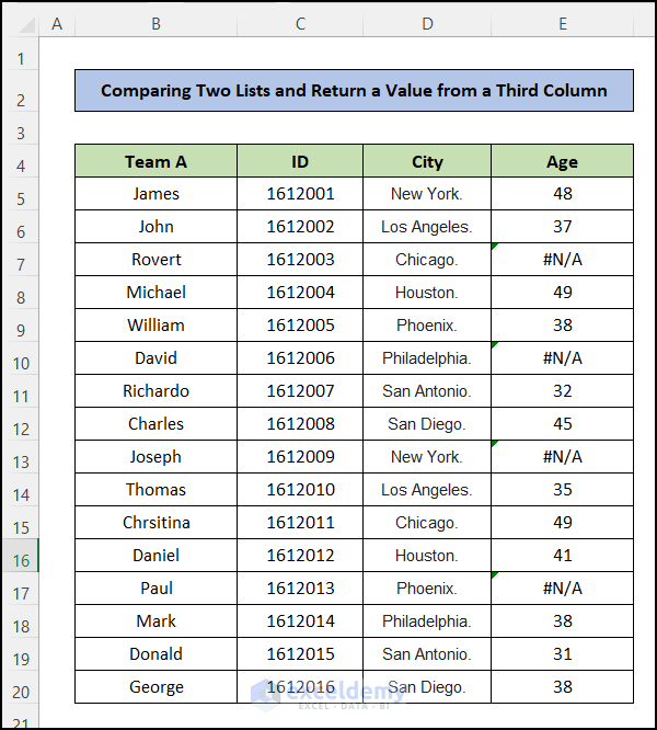
- We get the ages for the names that match the list in TeamA. For the mismatched names, we get an #N/A error.
Read More: How to Compare Three Columns and Return a Value in Excel
VLOOKUP for Multiple Columns in Different Sheets in Excel with One Return Only
We’re considering a situation with Item ID and Product Name of some products in a worksheet named W1 and Product Name and Price in another worksheet named W2. We’ll find the price of the product based on its ID.
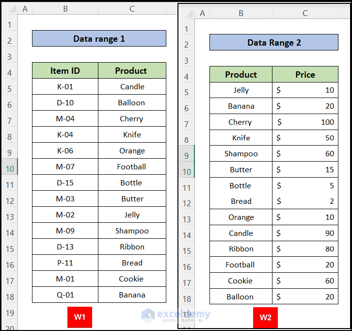
- Make a new sheet and list item IDs you want to find in column B starting with B5.
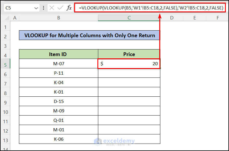
- Insert this formula into cell C5 of that sheet:
=VLOOKUP(VLOOKUP(B6,'W1'!B6:C19,2,FALSE),'W2'!B6:C19,2,FALSE)- Lookup_value is VLOOKUP(B6,’W1′!B6:C19,2,FALSE). This second “VLOOKUP” will pull the Item ID from the “W1”
- table_array: is ‘W2′!B6:C19.
- Col_index_num is 2
- [range_lookup]: we want the exact match (FALSE)
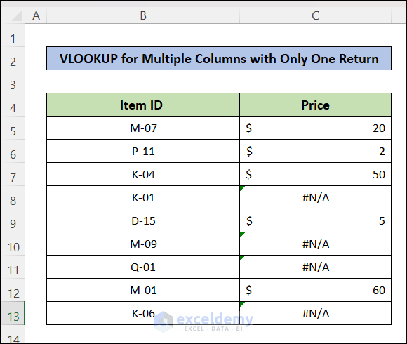
- Drag the Fill Handle icon to apply the formula to other cells of the column.
Download the Practice Workbook
<< Go Back to Columns | Compare | Learn Excel
Get FREE Advanced Excel Exercises with Solutions!

Good one.
Thanks for your feedback!
Hii
In sheet 1, column C (Owner Names) and Column D (Tenant names) are provided along with “Comments” in Column E for a city. And in sheet 2, owner names are provided in column F, and tenant names are in Column H, but comments are not provided.
Now I want, if in sheet1, any of the rows, the Owner name and tenant name exactly match with the owner’s name and tenant name in Sheet2 . then the comments should be copied from sheet 1 to sheet 2 in column O. In other words, if Column C & Column D (Sheet1) = Column F & Column H (Sheet 2), then from sheet 1 column E (Comments) should be pasted in Column O in the sheet 2.
Hope I have described my problem clearly, please help me to generate the formula for this.
Hello AVINASH! I have made a dataset as per your description and solved your problem. You can paste the following formula into the column O and the 3rd row to get the comment from sheet 1 when the criteria are met:
Try this for your dataset and let us know the outcome. Thank You!
I have selected a product in Column E of row 4 Sheet1 and I want the selected product to be searched in Column B of Product List and get the result in Column M of Sheet2
Hi Brijesh,
I have created a simplified solution below. Please follow them:
1. I am assuming that you have a Sheet1 like below:
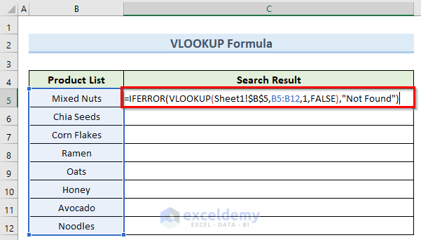
2. Now, go to the Sheet2 and insert the following formula in cell C5:
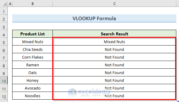
=IFERROR(VLOOKUP(Sheet1!$B$5,B5:B12,1,FALSE),"Not Found")3. Now, simply copy this formula down using Fill Handle and this should tell you whether the product in cell B5 inside Sheet1 exists in the Product List column or not.
Please help me with the below 2 requirements :
1. I need to compare two columns A & B in excel and find only the Newly Added names (Not the matched ones) in Column B after comparing them with column A.
2. Similary, I need to find the Removed Names which are missing in column B but they are available in column A.
Hope you help me with this asap.
Hello Harry,
Thank you for your comment! Here’s how you can achieve both requirements in Excel:
1. Find Newly Added Names in Column B (Not in Column A)
Use the following formula in a new column:
=IF(COUNTIF(A:A, B1) = 0, B1, “”)
This will display only the newly added names from Column B.
2. Find Removed Names in Column A (Not in Column B)
Use this formula in a new column:
=IF(COUNTIF(B:B, A1) = 0, A1, “”)
This will list the names in Column A that are missing in Column B.
Regards
ExcelDemy
Hello, I have 2 sheets. On the First sheet I have ID Numbers and a lot of data, on the Second Sheet I have the ID Numbers and the date they were built (not in the same order as the First sheet). I need to pull the Date Built from the Second sheet to next to its partnering ID Number on the First sheet.
I would really appreciate some direction.
Thank you,
Hello KJ,
You can absolutely achieve this using the VLOOKUP function. Since your ID Numbers are the common link between both sheets, VLOOKUP can help pull the “Date Built” from the second sheet to the first.
Here’s a step-by-step example:
1. Suppose your First Sheet is named DataSheet and the Second Sheet is BuildSheet.
2. In BuildSheet, column A has ID Numbers and column B has the corresponding Date Built.
3. In DataSheet, you want to pull the Date Built next to the ID Number in column A.
Use this formula in DataSheet (assuming ID is in A2):
=VLOOKUP(A2, BuildSheet!A:B, 2, FALSE)
This tells Excel to look up the ID from DataSheet!A2 in BuildSheet!A:A, and return the matching value from column B (the second column), where the Date Built is.
If you want to avoid errors in case an ID is missing, wrap it with IFERROR:
=IFERROR(VLOOKUP(A2, BuildSheet!A:B, 2, FALSE), “Not Found”)
Let me know if your sheet names or column structure are different—I’d be happy to adjust the formula for you!
Regards
ExcelDemy
So
BuildSheet = Build Log
DataSheet = Date Repair Built
And the Date in the Build Log is in column A and the ID is in column B.
I tried tweaking yours and I just kept breaking it….
Thank you again
Hello again!
Thanks for the clarification! Since in your Build Log sheet the Date is in column A and the ID is in column B, you’ll need to slightly adjust the VLOOKUP.
In your Date Repair Built sheet (where you have the ID and want to bring the Date Built next to it), use this formula:
=VLOOKUP(A2, ‘Build Log’!B:A, 2, FALSE)
Important:
Notice that I reversed the range to B:A because VLOOKUP always searches in the first column of the range you specify. So here:
B:B is where it looks for the ID,
and A:A is where it pulls the matching Date Built.
Also, if you want to avoid errors for missing IDs, you can use:
=IFERROR(VLOOKUP(A2, ‘Build Log’!B:A, 2, FALSE), “Not Found”)
This will show “Not Found” instead of an error if the ID doesn’t exist in the Build Log.
Let me know if you want me to walk you through a full working example too! You’re doing great!
Regards
ExcelDemy
Hello,
On worksheet 1, column A (Last Names) and column B (First names) – I need to figure out how to find the exact match on worksheet 2, column A (Last Name) and column B First Name) and then column C is location. Essentially I need to makes sure the first name and last names match on each worksheet and then figure out location they work at (location) on worksheet 1.
Hello Vanessa,
You can achieve this by using the VLOOKUP function with a helper column to combine the first and last names for an exact match. Here’s how you can do it:
Step 1: In both worksheets, create a new column (for example, Column D) that combines Last Name and First Name. Use this formula in cell D2 of both sheets:
=A2 & ” ” & B2
Step 2: Now, in Worksheet 1 (let’s say in cell C2), use the following formula to bring the location from Worksheet 2:
=VLOOKUP(D2, ‘Worksheet2’!D:C, 3, FALSE)
‘Worksheet2’!D:C assumes you have the combined names in Column D and location in Column C in Worksheet 2.
Adjust the column references as needed. It checks for an exact match of combined first and last names in both sheets and returns the location from Worksheet 2.
Regards
ExcelDemy