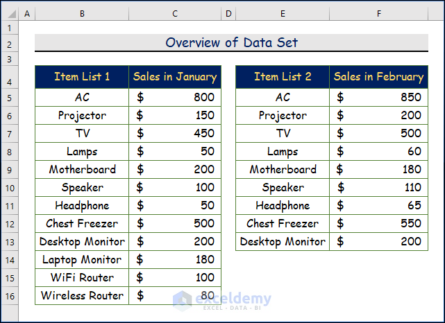
For illustration, we will use following sample dataset containing two lists of items.
Method 1 – Comparing Text in Two Columns For Matches in Rows
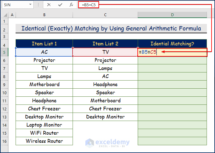
1.1 Identical (Exactly) Matching by Using General Arithmetic Formula
Steps:
- B5 is the cell of an item from Item List 1 and C5 is the cell of an item from Item List 2.
- Select the D5 cell.
- Add the following formula.
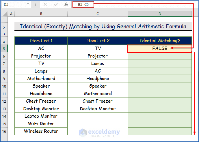
=B5=C5- Press ENTER.
- Excel will output the first identical match in the D5 cell.
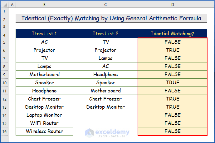
- Use the Fill Handle tool and drag it down from the D5 cell to the D16 cell.
- It will display all the identical matching as true and false.
1.2 Identical Matches and Differences Using IF Function
Steps:
- Choose the D5 cell.
- Apply the formula.
=IF(B5=C5,"Match","Not Match")- Hit ENTER.
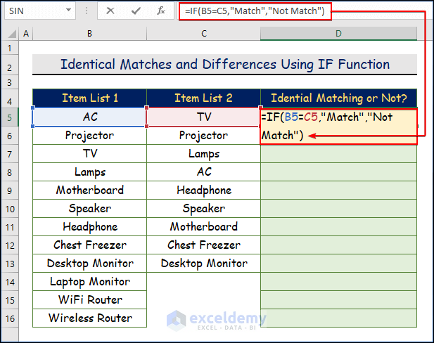
- You will get the result as NOT Match in the D5 cell.
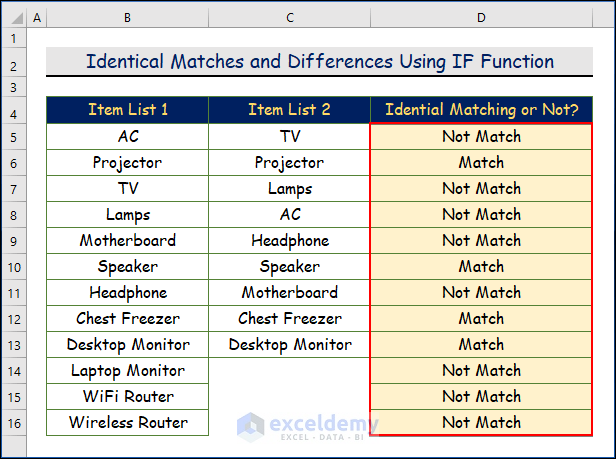
- Drag the Fill Handle tool down from the D5 cell to the D16 cell.
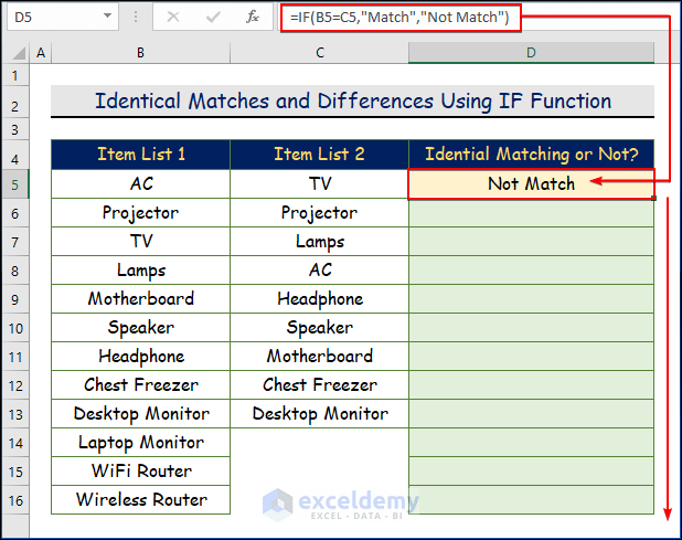
- You will get all the results.
1.3 Comparing Matches or Differences with Case-sensitive Analysis
Steps:
- In this image, we will color the given two rows to see the difference.
- Select cell D5.
- Apply the formula.
=IF(EXACT(B5,C5),"Match","Not Match")- Hit ENTER.
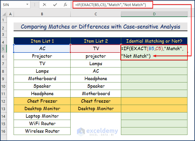
- You will see the result in the D5 cell.
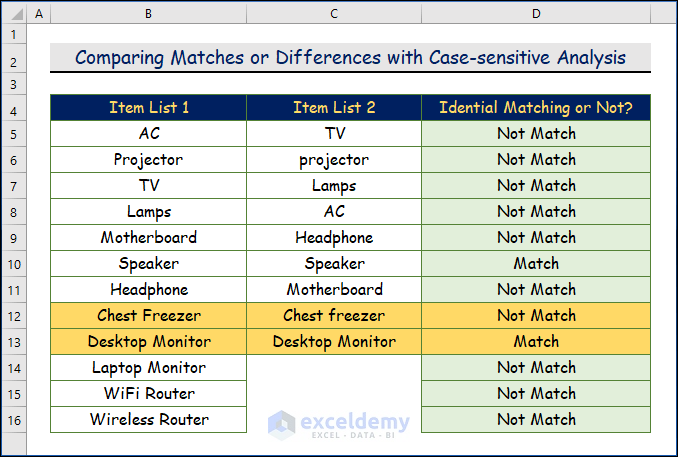
- Drag the Fill Handle tool from the D5 cell to the D16 cell.
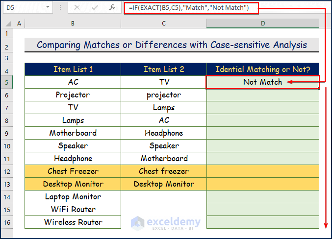
- Only the change in F of the Chest Freezer provides the result “Not Match”
Read More: Excel formula to compare two columns and return a value
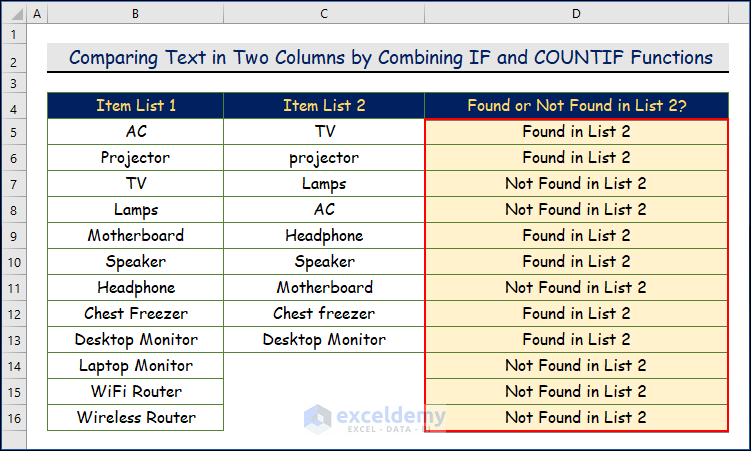
Method 2 – Compare Text in Two Columns by Combining IF and COUNTIF Functions in Excel
Steps:
- Select cell D5.
- Add the formula below. (C5:C13 is the cell range for item list 2, and B5 is the cell of an item from item list 1. If the IF function returns zero (Not Found in List 2) or 1 (Found in List 2).
=IF(COUNTIF($C5:$C13, $B5)=0, "Not Found in List 2", "Found in List 2")- Press ENTER.
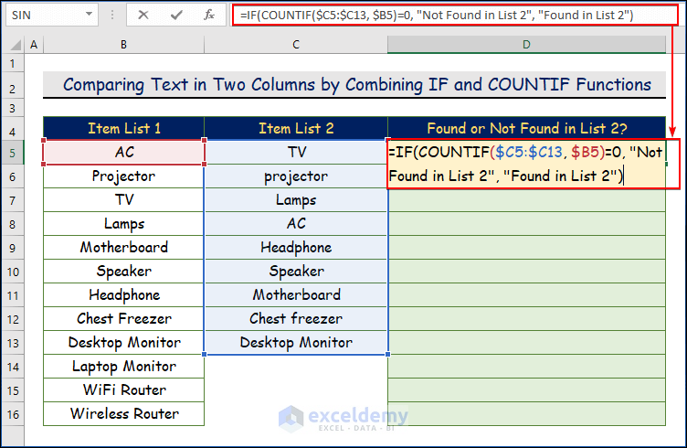
- You will see the result in cell D5.
- Use the Fill Handle tool and drag it down from the D5 cell to the D16 cell.
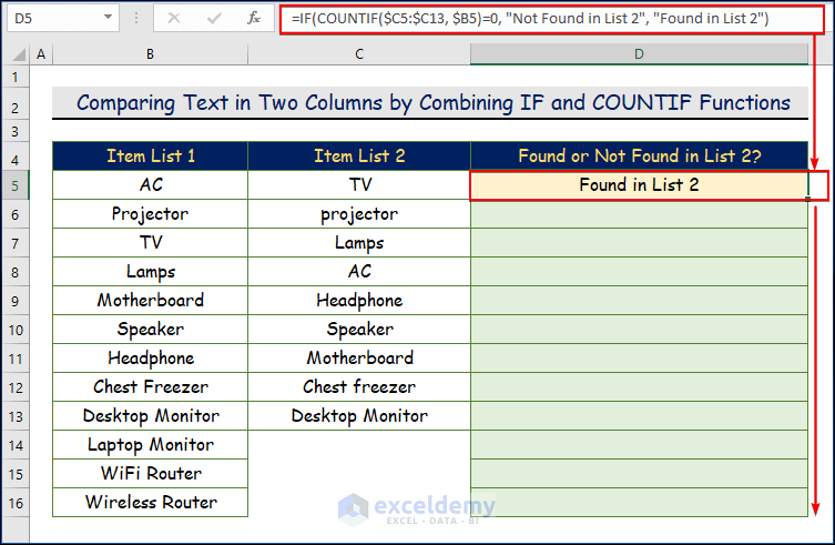
- You will get all the results as shown in this image.
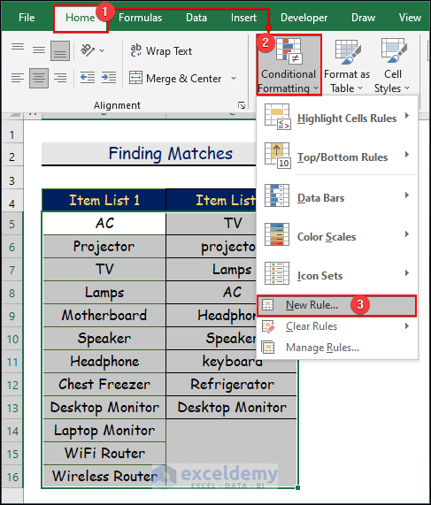
Method 3 – Applying Conditional Formatting to Compare Text in Two Columns for Matches and Differences
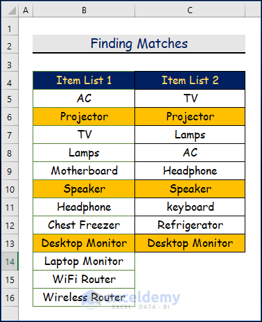
3.1 Finding Matches
Steps:
- Go to Home>Conditional Formatting>New Rule.
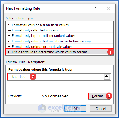
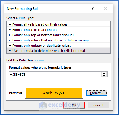
- Select Use a formula to determine which cells to format option and insert the formula in the blank space as in the following screenshot.
=$B5=$C5- Click on Format.
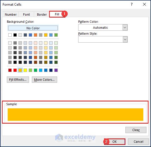
- Go to the Fill option, choose your desired color, and click OK.
- Click OK in the New Formatting Rule dialog box.
- You’ll get the following output. Only the speaker and desktop monitor are matched.
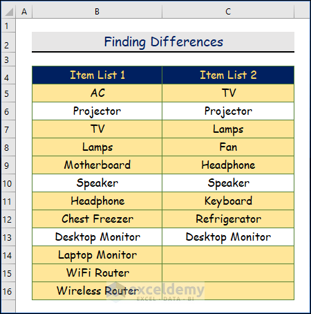
3.2 Finding Differences
Steps:
- Follow the same procedure as 3.1, but change the formula to this one.
=$B5<>$C5- You will get the following output.
Method 4 – Highlighting Duplicate or Unique Text to Compare in Two Columns Using Conditional Formatting
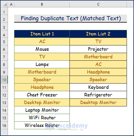
4.1 Finding Duplicate Text (Matched Text)
Steps:
- Select Home>Conditional Formatting>Highlight Cells Rules>Duplicate Values.
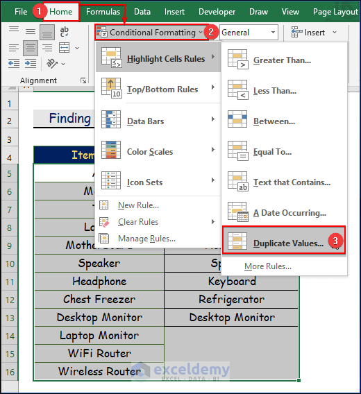
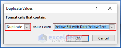
- Open the Duplicate Values.
- Preserve the default Duplicate option in the Format cells that contain it, change the values with option with a color of choice, and press OK.
- You’ll get the following output.
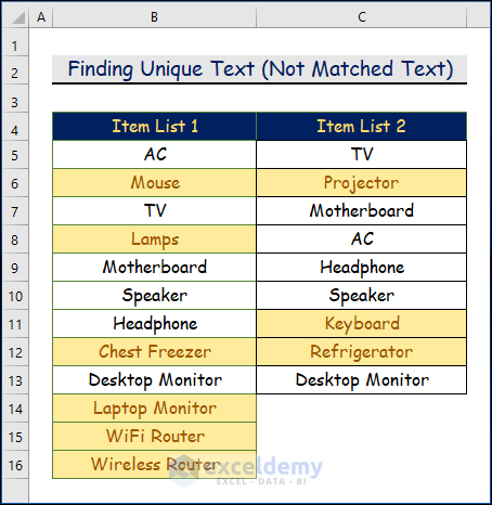
4.2 Finding Unique Text (Not Matched Text)
Steps:
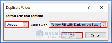
- Follow the previous steps till the dialog box Duplicate Values. In the dialog box, change the default option to Unique and press OK.
- You’ll get the following output.
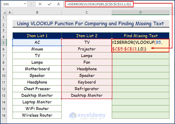
Method 5 – Using VLOOKUP Function For Comparing and Finding Missing Text in Excel
Steps:
- Select cell D5.
- Add the formula below.
=ISERROR(VLOOKUP(B5,$C$5:$C$13,1,0))- Press ENTER.
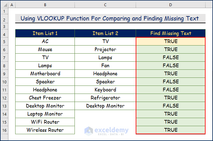
- You will see the first identical matching in the D5 cell.
- Use the Fill Handle tool and drag it down from the D5 cell to the D16 cell.

- You can see all the identical matching as true and false.
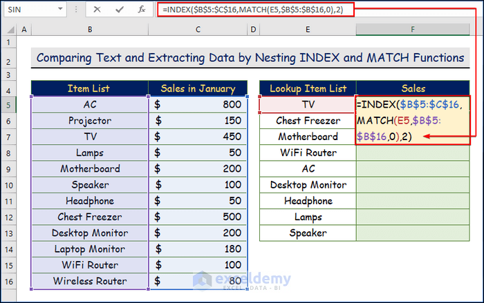
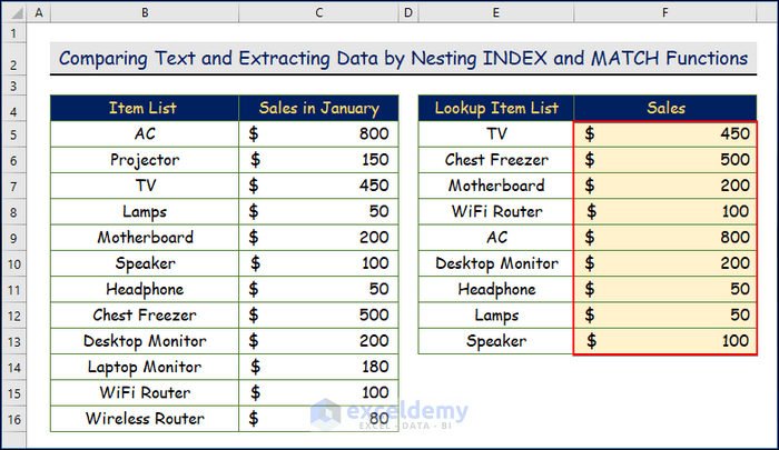
Method 6 – Comparing Text and Extracting Data by Nesting INDEX and MATCH Functions
Steps:
- Select cell D5.
- Add the following formula.
=INDEX($B$5:$C$16,MATCH(E5,$B$5:$B$16,0),2)- Press ENTER.
- B5:C16 is the list of items with their sales, E5 is a lookup item, B5:B16 is the item list, 0 is for the exact matching, and 2 is for the column index.
- You will see the Sales value in cell D5.
- Use the Fill Handle tool and drag it down from the D5 cell to the D16 cell.
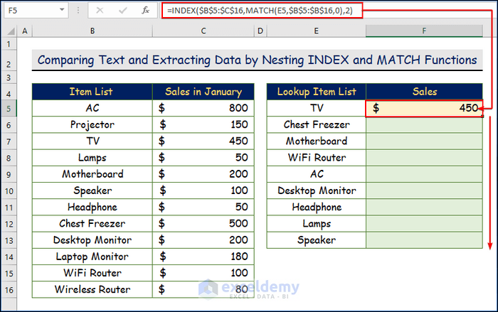
- You will get all the sales value.
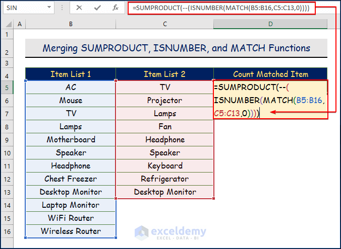
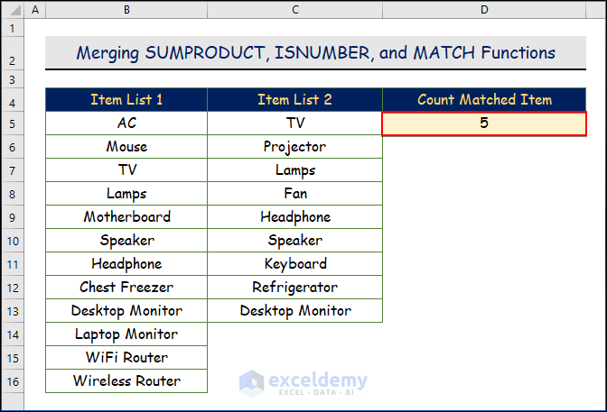
Method 7 – Merging SUMPRODUCT, ISNUMBER, and MATCH Functions to Compare Text in Two Columns with Counting Matches
Steps:
- Select cell D5.
- Add the following formula.
=SUMPRODUCT(--(ISNUMBER(MATCH(B5:B16,C5:C13,0))))- Hit ENTER.
- B5:B16 is the cell range for item list 1, and C5:C13 is for item list 2. The –ISNUMBER function is used to transform the output into numerical values.
- You will see the following output in the given image.
Download Practice Workbook
<< Go Back to Columns | Compare | Learn Excel
Get FREE Advanced Excel Exercises with Solutions!
