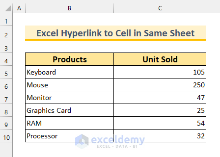
We’re going to show you 5 methods in Excel to create a hyperlink to a cell in the same sheet. To demonstrate our methods, we’ve taken a dataset with 2 columns: “Products”, and “Unit Sold”.
How to Hyperlink to Cell in Same Sheet in Excel: 5 Ways
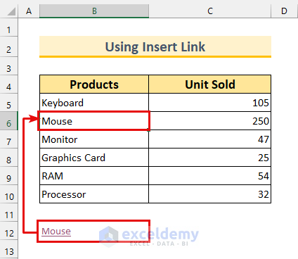
1. Using Insert Link in Excel to Hyperlink to Cell in Same Sheet
We’re going to use the “Insert Link” feature in Excel to Hyperlink to cell in the same Sheet.
Steps:
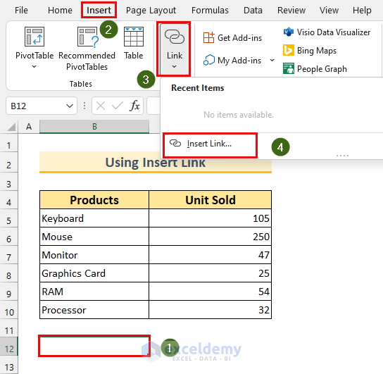
- Firstly, select cell B12.
- Secondly, from the Insert tab >>> Link >>> select Insert Link…
Then, the “Insert Hyperlink” dialog box will appear.
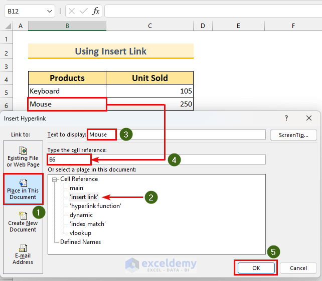
- Thirdly, select “Place in This Document”.
- Then, do these-
- Select ‘insert link’ from “Or select a place in this document:”
- Type “Mouse” in “Text to display:”
- Type B6 in “Type the cell reference:”.
- Finally, press OK.
We’ll see the text “Mouse” in cell B12 with link formatting.
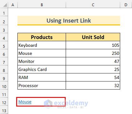
We can click on it, and it will select cell B6. Thus, we’ve created an Excel Hyperlink in the same Sheet.
Read More: How to Add Hyperlink to Another Sheet in Excel
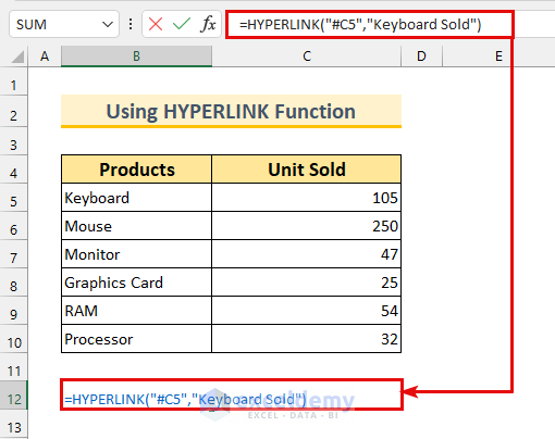
2. Hyperlink to Cell in Same Sheet by Implementing HYPERLINK Function
In this section, we’ll use the HYPERLINK function in Excel to create a Hyperlink to a cell in the same Sheet.
Steps:
- Firstly, type the following formula in cell B12.
=HYPERLINK("#C5","Keyboard Sold")The HYPERLINK function returns a clickable value. Here, we’ll get the link to cell C5. Moreover, we’ve put a hash (“#”) to indicate within this Sheet. Then, we’ll display the second part in cell B12 which is “Keyboard Sold”.
- Secondly, press ENTER.
After that, we’ll see the text “Keyboard Sold” appear in cell B12.
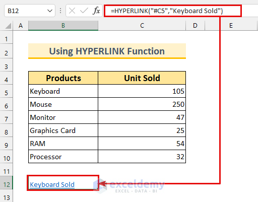
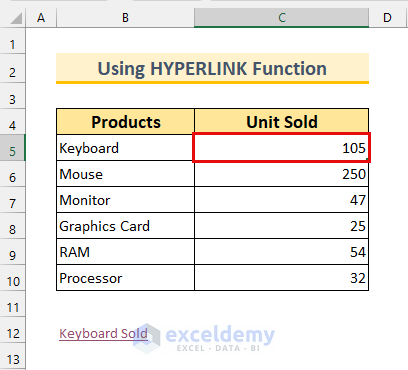
Again, we can click on this to go to cell C5. Therefore, we’ve shown you yet another method of linking to a cell in the same Sheet.
Read More: How to Hyperlink Multiple Cells in Excel
3. Using Combined Functions to Create Dynamic Hyperlink to Cell in Same Sheet
For the third method, we’ll use the ADDRESS, ROW, and HYPERLINK functions to create a dynamic link to a cell in the same Sheet. This means, that if we delete or insert rows or columns in the dataset, our formula will not break. Moreover, notice there is a blank row in our dataset.
Steps:
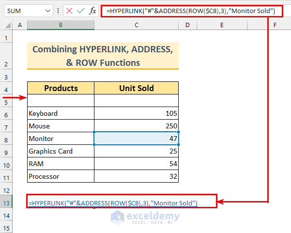
- Firstly, type the following formula in cell B13.
=HYPERLINK("#"&ADDRESS(ROW($C8),3),"Monitor Sold")Formula Breakdown
- ADDRESS(ROW($C8),3)
- Output: {“$C$8”}.
- The ROW function returns the row number of a cell. Cell C8 will return 8. Moreover, the ADDRESS function returns the location of a cell reference. Here, we’re denoting the C column by giving the value 3 in the formula. Thus we’ve got the output.
- Now, our formula reduces to, HYPERLINK(“#”&{“$C$8″},”Monitor Sold”)
- Output: “Monitor Sold”.
- The HYPERLINK function returns a clickable value. Here, we’ll get the link to cell C8. Moreover, we’ve put a hash (“#”) to indicate within this Sheet. Then, we’ll display the second part in cell B13 which is “Monitor Sold”.
- Secondly, press ENTER.
Then, we’ll see the output as described in the formula breakdown part.
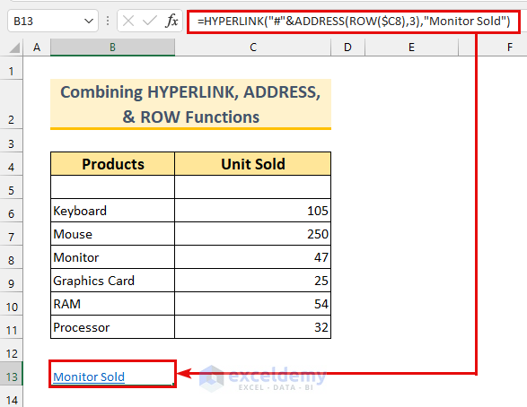
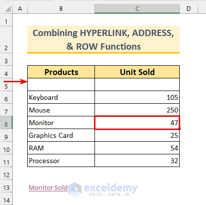
We can click on that value to go to cell C8. However, notice there is an empty row, we can delete blank rows to verify our dynamic formula still works.
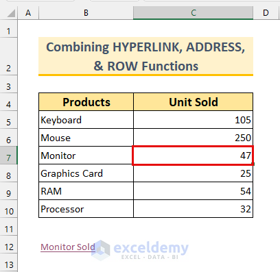
- Finally, remove Row 5.
If we click on the text “Monitor Sold”, we will select cell C7 now. Therefore, our formula works flawlessly.
Read More: How to Create Dynamic Hyperlink in Excel
4. Hyperlink to First Matched Cell in Same Sheet in Excel
In this section, we’ll use the CELL, INDEX, and MATCH functions to create a Hyperlink to the first matched values in the same Sheet.
Steps:
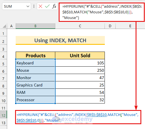
- Firstly, type the following formula in cell B12.
=HYPERLINK("#"&CELL("address",INDEX($B$5:$B$10,MATCH("Mouse",$B$5:$B$10,0))),"Mouse")Formula Breakdown
- MATCH(“Mouse”,$B$5:$B$10,0)
- Output: 2.
- The MATCH function is used to find the position of a value. Here, we’re looking for the value “Mouse” in the cell range B5:B10. Moreover, we’ve put the 0 for exact matching.
- Our INDEX portion becomes -> INDEX($B$5:$B$10,2)
- Output: “Mouse”.
- The INDEX function returns a value from a range. Here, we’re getting the value from the second row from the cell range B5:B10 which is cell B6.
- Then our formula in the CELL portion reduces to, CELL(“address”,”Mouse”)
- Output: “$B$6”.
- The CELL function returns information about a cell. Here, we’ve set out info_type as “address”. This will return the first occurrence of the text “Mouse” in our range which is cell B6.
- Finally, our formula reduces to, HYPERLINK(“#”&”$B$6″,”Mouse”)
- Output: “Mouse”.
- The HYPERLINK function returns a clickable value. Here, we’ll get the link to cell B6. Moreover, we’ve put a hash (“#”) to indicate within this Sheet. Then, we’ll display the second part in cell B12 which is “Mouse”.
- Secondly, press ENTER.
Then, we’ll see the output as described in the formula breakdown part.
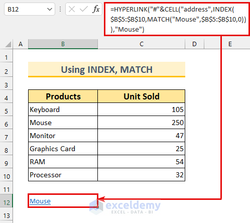
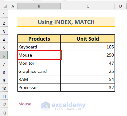
If we click on the text “Mouse”, we will select cell B6. Thus, we’ve shown you yet another formula to Hyperlink to a cell in the same Sheet.
5. Creating Hyperlink to Cell in Same Sheet from a Value
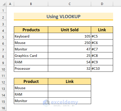
For the last method, we’re going to create Hyperlinks to cells in the same Sheet from values by using the HYPERLINK and VLOOKUP functions. Moreover, we’ve adjusted our dataset a bit for this.
Steps:
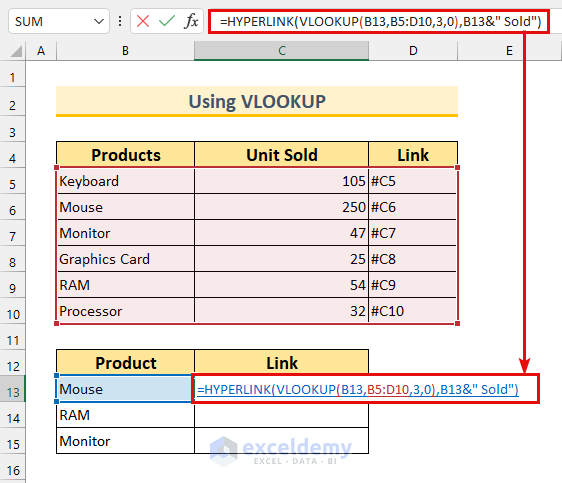
- Firstly, type the following formula in cell C13.
=HYPERLINK(VLOOKUP(B13,B5:D10,3,0),B13&" Sold")Formula Breakdown
- VLOOKUP(B13,B5:D10,3,0)
- Output: “#C6”.
- The VLOOKUP function returns a value from a range from the left side.
- Firstly, we’re looking for the value in cell B13 which is “Mouse”.
- Secondly, we’re setting our range in B5:D10.
- Thirdly, we’ll extract the value from column 3 which is the “Link” column.
- Finally, we’re putting 0 to find an exact match.
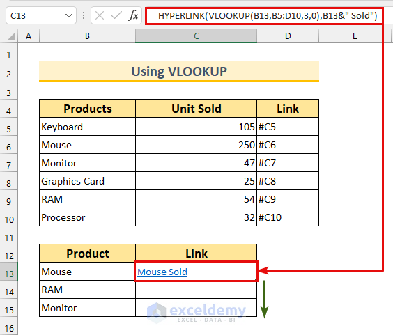
- Our formula reduces to, HYPERLINK(“#C6″,B13&” Sold”)
- Output: “Mouse Sold”.
- The HYPERLINK function returns a clickable value. Here, we’ll get the link to cell C6. Moreover, there is a hash (“#”) to indicate within this Sheet. Then, we’ll display the second part in cell B13 joined by the text “Sold” which is “Mouse Sold”.
- Secondly, press ENTER.
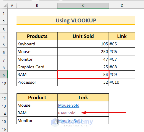
- Finally, use the Fill Handle to AutoFill the formula.
We can click on any of the Hyperlinks to go to their respective “Unit Sold” values in the dataset. In conclusion, we’ve achieved our goal of creating a Hyperlink to a cell in the same Sheet.
Read More: Excel Hyperlink to Cell in Another Sheet with VLOOKUP
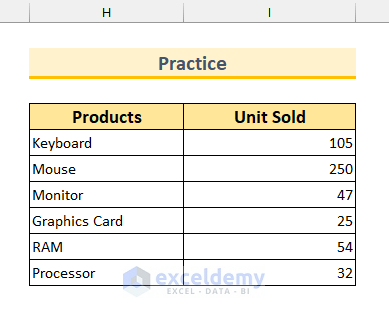
Practice Section
We’ve provided practice datasets for each method in the Excel file.
Download Practice Workbook
Conclusion
We’ve shown you 5 methods of Excel Hyperlink to cell in the same Sheet. If you face any difficulties in understanding any of the methods, feel free to comment below. Thanks for reading, keep excelling!
Related Articles
- How to Combine Text and Hyperlink in Excel Cell
- Excel Hyperlink to Another Sheet Based on Cell Value
- How to Create a Drop Down List Hyperlink to Another Sheet in Excel
- How to Edit Hyperlink in Excel
- How to Copy Hyperlink in Excel
- How to Convert Text to Hyperlink in Excel
- How to Create Button to Link to Another Sheet in Excel
<< Go Back To Create Hyperlink in Excel | Hyperlink in Excel | Linking in Excel | Learn Excel
Get FREE Advanced Excel Exercises with Solutions!
