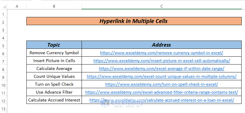
In this article, we will describe how to hyperlink multiple cells in Excel using 3 different methods. We’ll use the following sample dataset containing Excel-related topics and web addresses to demonstrate our methods.
Method 1 – Hyperlink Multiple Cells Using the Hyperlink Function
Using the HYPERLINK function we can easily create hyperlinks in Excel. Our dataset contains lengthy web addresses, so let’s link the addresses according to their topic name.
Steps:
- Enter the following formula in Cell D5:
=HYPERLINK(C5,B5)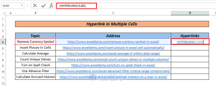
- Press ENTER.
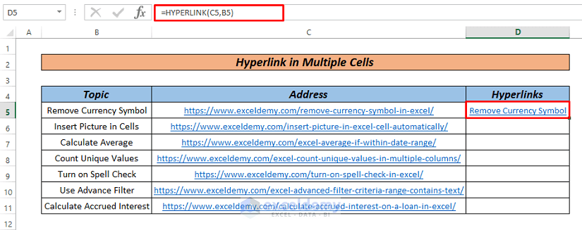
- Drag down the Fill Handle to AutoFill rest of the series.
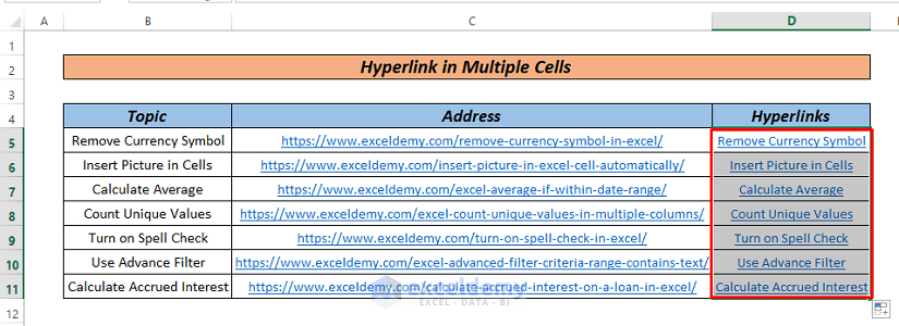
Hyperlinks are created for all the web links using their topic names as titles.
Read More: How to Create a Hyperlink in Excel
Method 2 – Hyperlink Links, Files, and Addresses in Excel
In addition to websites, we can also create hyperlinks for files and cells in Excel.
Steps:
- Click on cell C5 and press CTRL+K, or go to INSERT > Hyperlink.
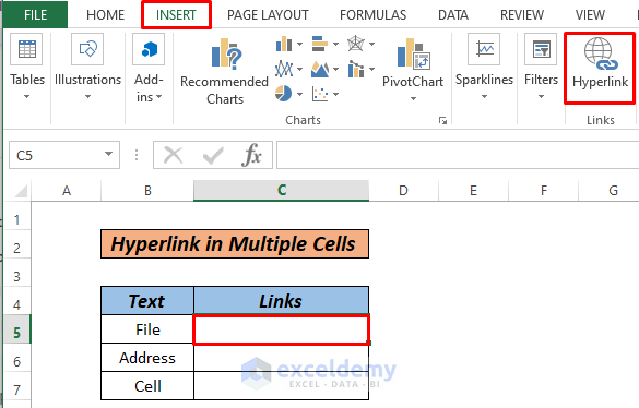
- Select any file, image, existing Excel file, Powerpoint etc. in the dialog box.
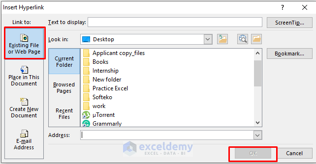
Here, we have selected an Excel file and renamed it in the Text to display box.
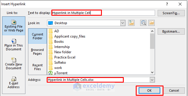
- Click OK.
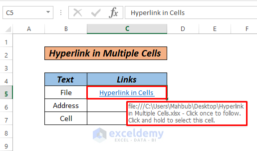
. A hyperlink to the file is created. Clicking this link will automatically open the linked file.
- To create web links, press CTRL+K and do the following:
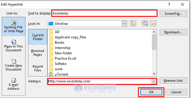
Here, we have created a link for our website exceldemy.com.
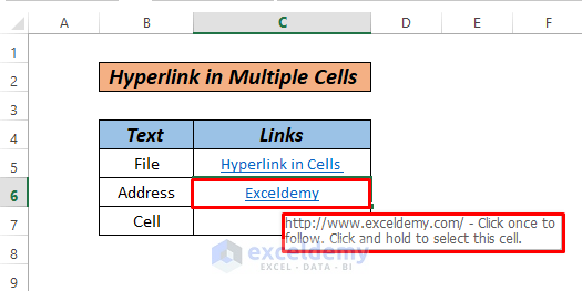
- To link to a cell in Excel, do the following after pressing CTRL+K:
The cell will look like the following image.
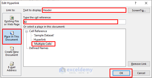
Now, we will create a hyperlink for different sheets. Suppose, we want to create a hyperlink that will take us to the location of topics in our Excel sheet.
- Press CTRL+K and do the following:
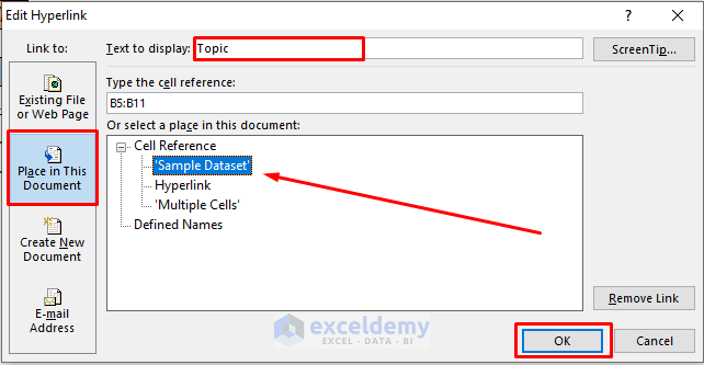
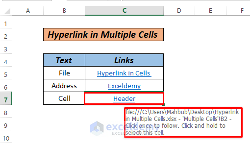
Here, we selected the Sample Dataset sheet. Our dataset will look like the following image:
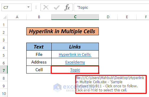
Clicking on this hyperlink will take us to the topic name range in our dataset in the active workbook file.

Read More: Excel Hyperlink with Shortcut Key
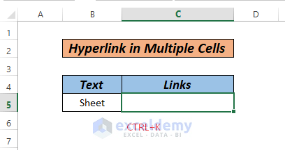
Method 3 – Creating a Hyperlink for a Cell Range Using Name Range
Here, we will apply Defined Names to create hyperlinks.
Steps:
- Select the range to be hyperlinked and go to Formulas > Defined Names.
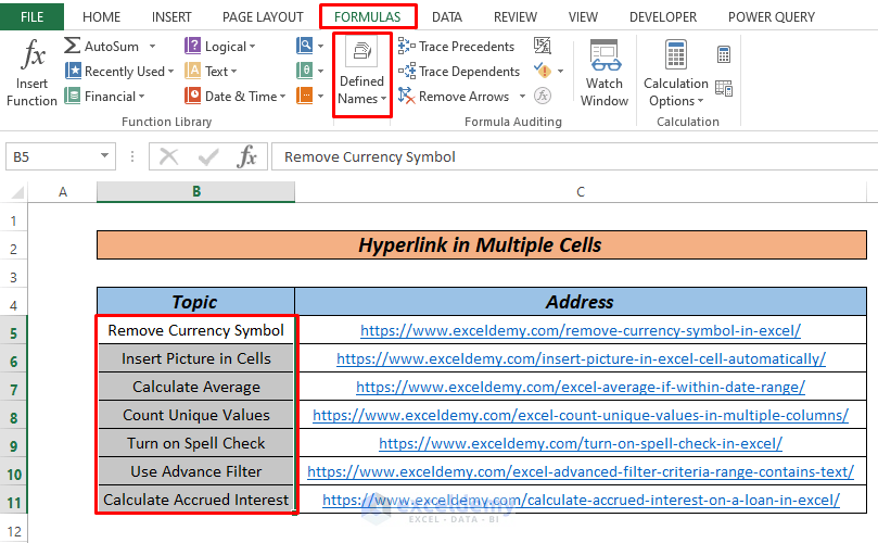
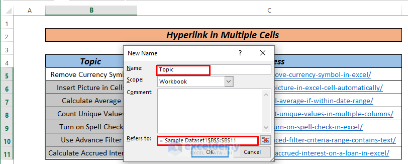
The New Name dialog box will pop up with the selected range pre-selected.
- Define the range name and click OK.
- Select the cell where the hyperlink will be inserted and press CTRL+K.
- Select the name we just defined.
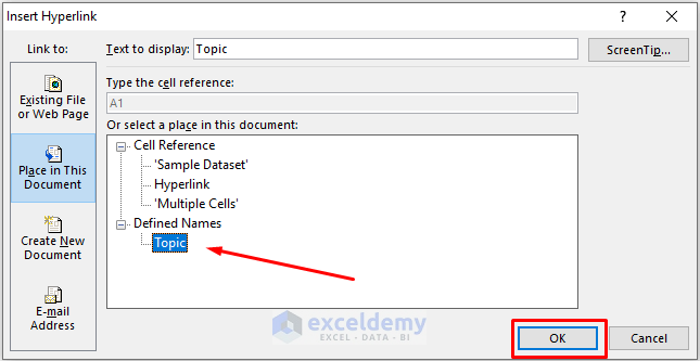
- Click OK to return the following result:
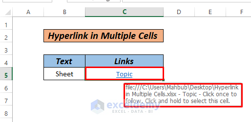
If you click the link, it will take you to the location where the multiple cells are hyperlinked.
Read More: How to Hyperlink to Cell in Excel
Download Practice Workbook
Related Articles
- How to Activate Multiple Hyperlinks in Excel
- How to Fix Broken Hyperlinks in Excel
- How to Hyperlink Multiple PDF Files in Excel
- How to Link Files in Excel
- How to Create Button Without Macro in Excel
<< Go Back To Create Hyperlink in Excel | Hyperlink in Excel | Linking in Excel | Learn Excel
Get FREE Advanced Excel Exercises with Solutions!
